Augment data with information from a(n) lm object

Augment accepts a model object and a dataset and adds information about each observation in the dataset. Most commonly, this includes predicted values in the .fitted column, residuals in the .resid column, and standard errors for the fitted values in a .se.fit column. New columns always begin with a . prefix to avoid overwriting columns in the original dataset.

Users may pass data to augment via either the data argument or the newdata argument. If the user passes data to the data argument, it must be exactly the data that was used to fit the model object. Pass datasets to newdata to augment data that was not used during model fitting. This still requires that all columns used to fit the model are present.

Augment will often behave differently depending on whether data or newdata is given. This is because there is often information associated with training observations (such as influences or related) measures that is not meaningfully defined for new observations.

For convenience, many augment methods provide default data arguments, so that augment(fit) will return the augmented training data. In these cases, augment tries to reconstruct the original data based on the model object with varying degrees of success.

The augmented dataset is always returned as a tibble::tibble with the same number of rows as the passed dataset. This means that the passed data must be coercible to a tibble. At this time, tibbles do not support matrix-columns. This means you should not specify a matrix of covariates in a model formula during the original model fitting process, and that splines::ns(), stats::poly() and survival::Surv() objects are not supported in input data. If you encounter errors, try explicitly passing a tibble, or fitting the original model on data in a tibble.

We are in the process of defining behaviors for models fit with various na.action arguments, but make no guarantees about behavior when data is missing at this time.

# S3 method for lm
augment(x, data = model.frame(x), newdata = NULL, se_fit = FALSE, ...)

Arguments

x	An `lm` object created by `stats::lm()`.
data	A base::data.frame or `tibble::tibble()` containing the original data that was used to produce the object `x`. Defaults to `stats::model.frame(x)` so that `augment(my_fit)` returns the augmented original data. Do not pass new data to the `data` argument. Augment will report information such as influence and cooks distance for data passed to the `data` argument. These measures are only defined for the original training data.
newdata	A `base::data.frame()` or `tibble::tibble()` containing all the original predictors used to create `x`. Defaults to `NULL`, indicating that nothing has been passed to `newdata`. If `newdata` is specified, the `data` argument will be ignored.
se_fit	Logical indicating whether or not a `.se.fit` column should be added to the augmented output. For some models, this calculation can be somwhat time-consuming. Defaults to `FALSE`.
...	Additional arguments. Not used. Needed to match generic signature only. Cautionary note: Misspelled arguments will be absorbed in `...`, where they will be ignored. If the misspelled argument has a default value, the default value will be used. For example, if you pass `conf.lvel = 0.9`, all computation will proceed using `conf.level = 0.95`. Additionally, if you pass `newdata = my_tibble` to an `augment()` method that does not accept a `newdata` argument, it will use the default value for the `data` argument.

Details

When the modeling was performed with na.action = "na.omit" (as is the typical default), rows with NA in the initial data are omitted entirely from the augmented data frame. When the modeling was performed with na.action = "na.exclude", one should provide the original data as a second argument, at which point the augmented data will contain those rows (typically with NAs in place of the new columns). If the original data is not provided to augment() and na.action = "na.exclude", a warning is raised and the incomplete rows are dropped.

Some unusual lm objects, such as rlm from MASS, may omit .cooksd and .std.resid. gam from mgcv omits .sigma.

When newdata is supplied, only returns .fitted, .resid and .se.fit columns.

Value

A tibble::tibble() with columns:

.cooksd

Cooks distance.

.fitted

Fitted or predicted value.

.hat

Diagonal of the hat matrix.

.resid

The difference between observed and fitted values.

.se.fit

Standard errors of fitted values.

.sigma

Estimated residual standard deviation when corresponding observation is dropped from model.

.std.resid

Standardised residuals.

Examples


library(ggplot2)
library(dplyr)

mod <- lm(mpg ~ wt + qsec, data = mtcars)

tidy(mod)
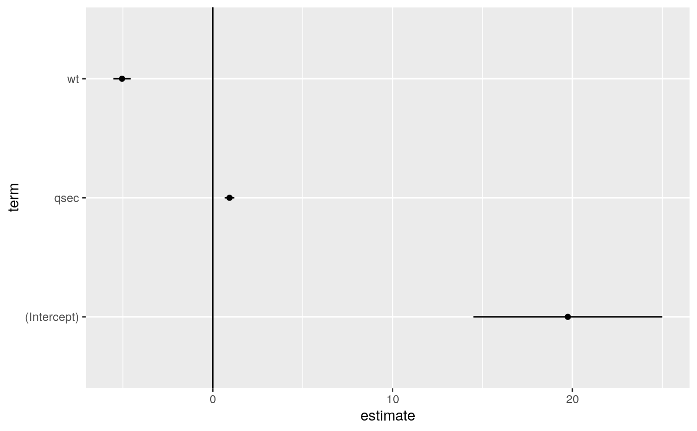
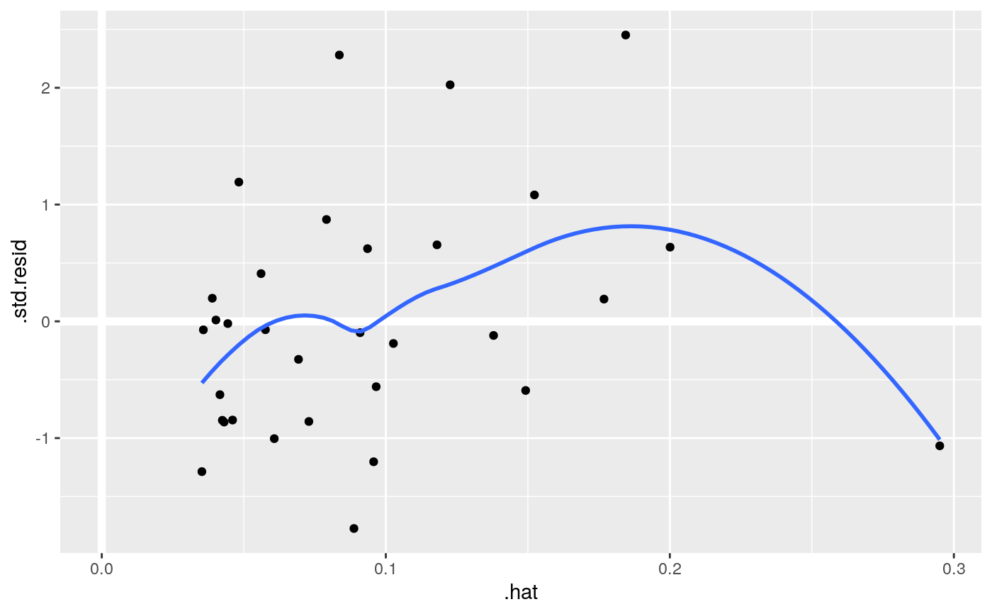
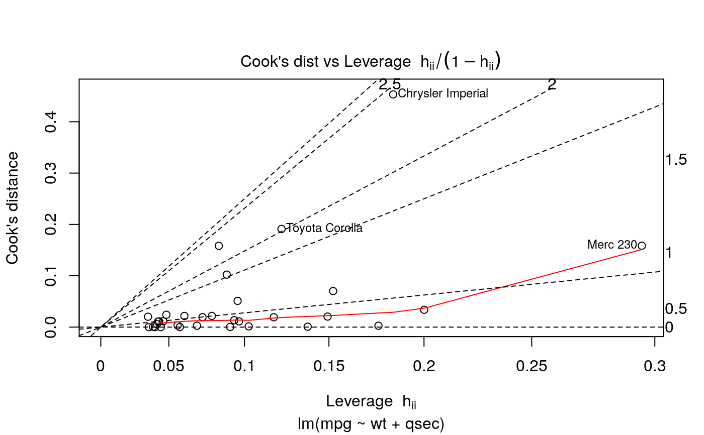
#> # A tibble: 3 x 5
#>   term        estimate std.error statistic  p.value
#>   <chr>          <dbl>     <dbl>     <dbl>    <dbl>
#> 1 (Intercept)   19.7       5.25       3.76 7.65e- 4
#> 2 wt            -5.05      0.484    -10.4  2.52e-11
#> 3 qsec           0.929     0.265      3.51 1.50e- 3
glance(mod)
#> # A tibble: 1 x 12
#>   r.squared adj.r.squared sigma statistic  p.value    df logLik   AIC   BIC
#>       <dbl>         <dbl> <dbl>     <dbl>    <dbl> <dbl>  <dbl> <dbl> <dbl>
#> 1     0.826         0.814  2.60      69.0 9.39e-12     2  -74.4  157.  163.
#> # … with 3 more variables: deviance <dbl>, df.residual <int>, nobs <int>

# coefficient plot
d <- tidy(mod) %>%
  mutate(
    low = estimate - std.error,
    high = estimate + std.error
  )

ggplot(d, aes(estimate, term, xmin = low, xmax = high, height = 0)) +
  geom_point() +
  geom_vline(xintercept = 0) +
  geom_errorbarh()

augment(mod)
#> # A tibble: 32 x 10
#>    .rownames    mpg    wt  qsec .fitted  .resid .std.resid   .hat .sigma .cooksd
#>    <chr>      <dbl> <dbl> <dbl>   <dbl>   <dbl>      <dbl>  <dbl>  <dbl>   <dbl>
#>  1 Mazda RX4   21    2.62  16.5    21.8 -0.815     -0.325  0.0693   2.64 2.63e-3
#>  2 Mazda RX4…  21    2.88  17.0    21.0 -0.0482    -0.0190 0.0444   2.64 5.59e-6
#>  3 Datsun 710  22.8  2.32  18.6    25.3 -2.53      -1.00   0.0607   2.60 2.17e-2
#>  4 Hornet 4 …  21.4  3.22  19.4    21.6 -0.181     -0.0716 0.0576   2.64 1.05e-4
#>  5 Hornet Sp…  18.7  3.44  17.0    18.2  0.504      0.198  0.0389   2.64 5.29e-4
#>  6 Valiant     18.1  3.46  20.2    21.1 -2.97      -1.20   0.0957   2.58 5.10e-2
#>  7 Duster 360  14.3  3.57  15.8    16.4 -2.14      -0.857  0.0729   2.61 1.93e-2
#>  8 Merc 240D   24.4  3.19  20      22.2  2.17       0.872  0.0791   2.61 2.18e-2
#>  9 Merc 230    22.8  3.15  22.9    25.1 -2.32      -1.07   0.295    2.59 1.59e-1
#> 10 Merc 280    19.2  3.44  18.3    19.4 -0.185     -0.0728 0.0358   2.64 6.55e-5
#> # … with 22 more rows
augment(mod, mtcars)
#> # A tibble: 32 x 18
#>    .rownames   mpg   cyl  disp    hp  drat    wt  qsec    vs    am  gear  carb
#>    <chr>     <dbl> <dbl> <dbl> <dbl> <dbl> <dbl> <dbl> <dbl> <dbl> <dbl> <dbl>
#>  1 Mazda RX4  21       6  160    110  3.9   2.62  16.5     0     1     4     4
#>  2 Mazda RX…  21       6  160    110  3.9   2.88  17.0     0     1     4     4
#>  3 Datsun 7…  22.8     4  108     93  3.85  2.32  18.6     1     1     4     1
#>  4 Hornet 4…  21.4     6  258    110  3.08  3.22  19.4     1     0     3     1
#>  5 Hornet S…  18.7     8  360    175  3.15  3.44  17.0     0     0     3     2
#>  6 Valiant    18.1     6  225    105  2.76  3.46  20.2     1     0     3     1
#>  7 Duster 3…  14.3     8  360    245  3.21  3.57  15.8     0     0     3     4
#>  8 Merc 240D  24.4     4  147.    62  3.69  3.19  20       1     0     4     2
#>  9 Merc 230   22.8     4  141.    95  3.92  3.15  22.9     1     0     4     2
#> 10 Merc 280   19.2     6  168.   123  3.92  3.44  18.3     1     0     4     4
#> # … with 22 more rows, and 6 more variables: .fitted <dbl>, .resid <dbl>,
#> #   .std.resid <dbl>, .hat <dbl>, .sigma <dbl>, .cooksd <dbl>

# predict on new data
newdata <- mtcars %>%
  head(6) %>%
  mutate(wt = wt + 1)
augment(mod, newdata = newdata)
#> # A tibble: 6 x 13
#>     mpg   cyl  disp    hp  drat    wt  qsec    vs    am  gear  carb .fitted
#>   <dbl> <dbl> <dbl> <dbl> <dbl> <dbl> <dbl> <dbl> <dbl> <dbl> <dbl>   <dbl>
#> 1  21       6   160   110  3.9   3.62  16.5     0     1     4     4    16.8
#> 2  21       6   160   110  3.9   3.88  17.0     0     1     4     4    16.0
#> 3  22.8     4   108    93  3.85  3.32  18.6     1     1     4     1    20.3
#> 4  21.4     6   258   110  3.08  4.22  19.4     1     0     3     1    16.5
#> 5  18.7     8   360   175  3.15  4.44  17.0     0     0     3     2    13.1
#> 6  18.1     6   225   105  2.76  4.46  20.2     1     0     3     1    16.0
#> # … with 1 more variable: .resid <dbl>

au <- augment(mod, data = mtcars)

ggplot(au, aes(.hat, .std.resid)) +
  geom_vline(size = 2, colour = "white", xintercept = 0) +
  geom_hline(size = 2, colour = "white", yintercept = 0) +
  geom_point() +
  geom_smooth(se = FALSE)
#> `geom_smooth()` using method = 'loess' and formula 'y ~ x'

plot(mod, which = 6)
ggplot(au, aes(.hat, .cooksd)) +
  geom_vline(xintercept = 0, colour = NA) +
  geom_abline(slope = seq(0, 3, by = 0.5), colour = "white") +
  geom_smooth(se = FALSE) +
  geom_point()
#> `geom_smooth()` using method = 'loess' and formula 'y ~ x'

# column-wise models
a <- matrix(rnorm(20), nrow = 10)
b <- a + rnorm(length(a))
result <- lm(b ~ a)
tidy(result)
#> # A tibble: 6 x 6
#>   response term        estimate std.error statistic p.value
#>   <chr>    <chr>          <dbl>     <dbl>     <dbl>   <dbl>
#> 1 Y1       (Intercept)  -0.233      0.258   -0.904  0.396  
#> 2 Y1       a1            0.929      0.214    4.35   0.00336
#> 3 Y1       a2            0.0269     0.316    0.0852 0.934  
#> 4 Y2       (Intercept)   0.224      0.271    0.827  0.435  
#> 5 Y2       a1            0.161      0.225    0.716  0.497  
#> 6 Y2       a2            1.50       0.333    4.50   0.00279

Augment data with information from a(n) lm object

Arguments

Details

See also

Value

Examples