Tidy a(n) irlba object masquerading as list

Broom tidies a number of lists that are effectively S3 objects without a class attribute. For example, stats::optim(), svd() and akima::interp() produce consistent output, but because they do not have a class attribute, they cannot be handled by S3 dispatch.

These functions look at the elements of a list and determine if there is an appropriate tidying method to apply to the list. Those tidiers are themselves are implemented as functions of the form tidy_<function> or glance_<function> and are not exported (but they are documented!).

If no appropriate tidying method is found, throws an error.

tidy_irlba(x, ...)

Arguments

x

A list returned from irlba::irlba().

...

Additional arguments. Not used. Needed to match generic signature only. Cautionary note: Misspelled arguments will be absorbed in ..., where they will be ignored. If the misspelled argument has a default value, the default value will be used. For example, if you pass conf.lvel = 0.9, all computation will proceed using conf.level = 0.95. Additionally, if you pass newdata = my_tibble to an augment() method that does not accept a newdata argument, it will use the default value for the data argument.

Value

A tibble::tibble with columns depending on the component of PCA being tidied.

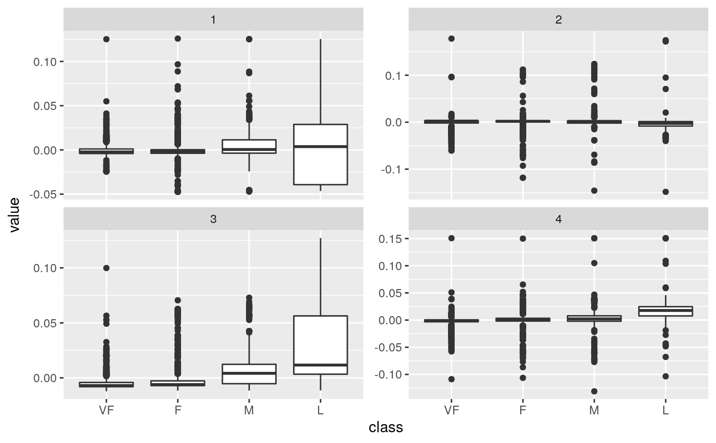
If matrix is "u", "samples", "scores", or "x" each row in the tidied output corresponds to the original data in PCA space. The columns are:

row

ID of the original observation (i.e. rowname from original data).

PC

Integer indicating a principal component.

value

The score of the observation for that particular principal component. That is, the location of the observation in PCA space.

If matrix is "v", "rotation", "loadings" or "variables", each row in the tidied output corresponds to information about the principle components in the original space. The columns are:

row

The variable labels (colnames) of the data set on which PCA was performed

PC

An integer vector indicating the principal component

value

The value of the eigenvector (axis score) on the indicated principal component

If matrix is "d", "eigenvalues" or "pcs", the columns are:

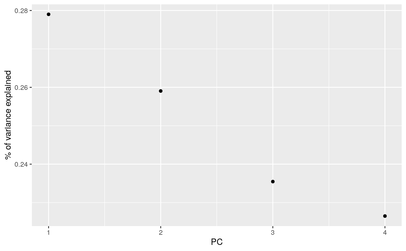
PC

An integer vector indicating the principal component

std.dev

Standard deviation explained by this PC

percent

Fraction of variation explained by this component

cumulative

Cumulative fraction of variation explained by principle components up to this component.

Details

A very thin wrapper around tidy_svd().

See also

tidy(), irlba::irlba()

Other list tidiers: glance_optim(), list_tidiers, tidy_optim(), tidy_svd(), tidy_xyz()

Other svd tidiers: augment.prcomp(), tidy.prcomp(), tidy_svd()

Examples

library(modeldata)
data(hpc_data)

mat <- scale(as.matrix(hpc_data[, 2:5]))
s <- svd(mat)

tidy_u <- tidy(s, matrix = "u")
#> New names:
#> * `` -> ...1
#> * `` -> ...2
#> * `` -> ...3
#> * `` -> ...4
tidy_u
#> # A tibble: 17,324 x 3
#>      row    PC    value
#>    <int> <dbl>    <dbl>
#>  1     1     1  0.00403
#>  2     2     1 -0.00436
#>  3     3     1 -0.00196
#>  4     4     1 -0.00444
#>  5     5     1 -0.00437
#>  6     6     1 -0.00437
#>  7     7     1 -0.00431
#>  8     8     1 -0.00436
#>  9     9     1 -0.00434
#> 10    10     1 -0.00440
#> # … with 17,314 more rows

tidy_d <- tidy(s, matrix = "d")
tidy_d
#> # A tibble: 4 x 4
#>      PC std.dev percent cumulative
#>   <int>   <dbl>   <dbl>      <dbl>
#> 1     1    69.5   0.279      0.279
#> 2     2    67.0   0.259      0.538
#> 3     3    63.9   0.235      0.774
#> 4     4    62.6   0.226      1.00 

tidy_v <- tidy(s, matrix = "v")
#> New names:
#> * `` -> ...1
#> * `` -> ...2
#> * `` -> ...3
#> * `` -> ...4
tidy_v
#> # A tibble: 16 x 3
#>    column    PC   value
#>     <int> <dbl>   <dbl>
#>  1      1     1  0.657 
#>  2      2     1  0.409 
#>  3      3     1 -0.577 
#>  4      4     1  0.262 
#>  5      1     2 -0.0142
#>  6      2     2 -0.650 
#>  7      3     2 -0.137 
#>  8      4     2  0.747 
#>  9      1     3  0.302 
#> 10      2     3  0.332 
#> 11      3     3  0.779 
#> 12      4     3  0.438 
#> 13      1     4  0.690 
#> 14      2     4 -0.548 
#> 15      3     4  0.205 
#> 16      4     4 -0.426 

library(ggplot2)
library(dplyr)

ggplot(tidy_d, aes(PC, percent)) +
  geom_point() +
  ylab("% of variance explained")

tidy_u %>%
  mutate(class = hpc_data$class[row]) %>%
  ggplot(aes(class, value)) +
  geom_boxplot() +
  facet_wrap(~PC, scale = "free_y")