Tidy summarizes information about the components of a model. A model component might be a single term in a regression, a single hypothesis, a cluster, or a class. Exactly what tidy considers to be a model component varies across models but is usually self-evident. If a model has several distinct types of components, you will need to specify which components to return.
# S3 method for nlrq
augment(x, data = NULL, newdata = NULL, ...)
Arguments
- x
A
nlrqobject returned fromquantreg::nlrq().- data
A base::data.frame or
tibble::tibble()containing the original data that was used to produce the objectx. Defaults tostats::model.frame(x)so thataugment(my_fit)returns the augmented original data. Do not pass new data to thedataargument. Augment will report information such as influence and cooks distance for data passed to thedataargument. These measures are only defined for the original training data.- newdata
A
base::data.frame()ortibble::tibble()containing all the original predictors used to createx. Defaults toNULL, indicating that nothing has been passed tonewdata. Ifnewdatais specified, thedataargument will be ignored.- ...
Additional arguments. Not used. Needed to match generic signature only. Cautionary note: Misspelled arguments will be absorbed in
..., where they will be ignored. If the misspelled argument has a default value, the default value will be used. For example, if you passconf.lvel = 0.9, all computation will proceed usingconf.level = 0.95. Additionally, if you passnewdata = my_tibbleto anaugment()method that does not accept anewdataargument, it will use the default value for thedataargument.
See also
Other quantreg tidiers:
augment.rqs(),
augment.rq(),
glance.nlrq(),
glance.rq(),
tidy.nlrq(),
tidy.rqs(),
tidy.rq()
Examples
# fit model
n <- nls(mpg ~ k * e^wt, data = mtcars, start = list(k = 1, e = 2))
# summarize model fit with tidiers + visualization
tidy(n)
#> # A tibble: 2 × 5
#> term estimate std.error statistic p.value
#> <chr> <dbl> <dbl> <dbl> <dbl>
#> 1 k 49.7 3.79 13.1 5.96e-14
#> 2 e 0.746 0.0199 37.5 8.86e-27
augment(n)
#> # A tibble: 32 × 4
#> mpg wt .fitted .resid
#> <dbl> <dbl> <dbl> <dbl>
#> 1 21 2.62 23.0 -2.01
#> 2 21 2.88 21.4 -0.352
#> 3 22.8 2.32 25.1 -2.33
#> 4 21.4 3.22 19.3 2.08
#> 5 18.7 3.44 18.1 0.611
#> 6 18.1 3.46 18.0 0.117
#> 7 14.3 3.57 17.4 -3.11
#> 8 24.4 3.19 19.5 4.93
#> 9 22.8 3.15 19.7 3.10
#> 10 19.2 3.44 18.1 1.11
#> # … with 22 more rows
glance(n)
#> # A tibble: 1 × 9
#> sigma isConv finTol logLik AIC BIC deviance df.residual nobs
#> <dbl> <lgl> <dbl> <dbl> <dbl> <dbl> <dbl> <int> <int>
#> 1 2.67 TRUE 0.00000204 -75.8 158. 162. 214. 30 32
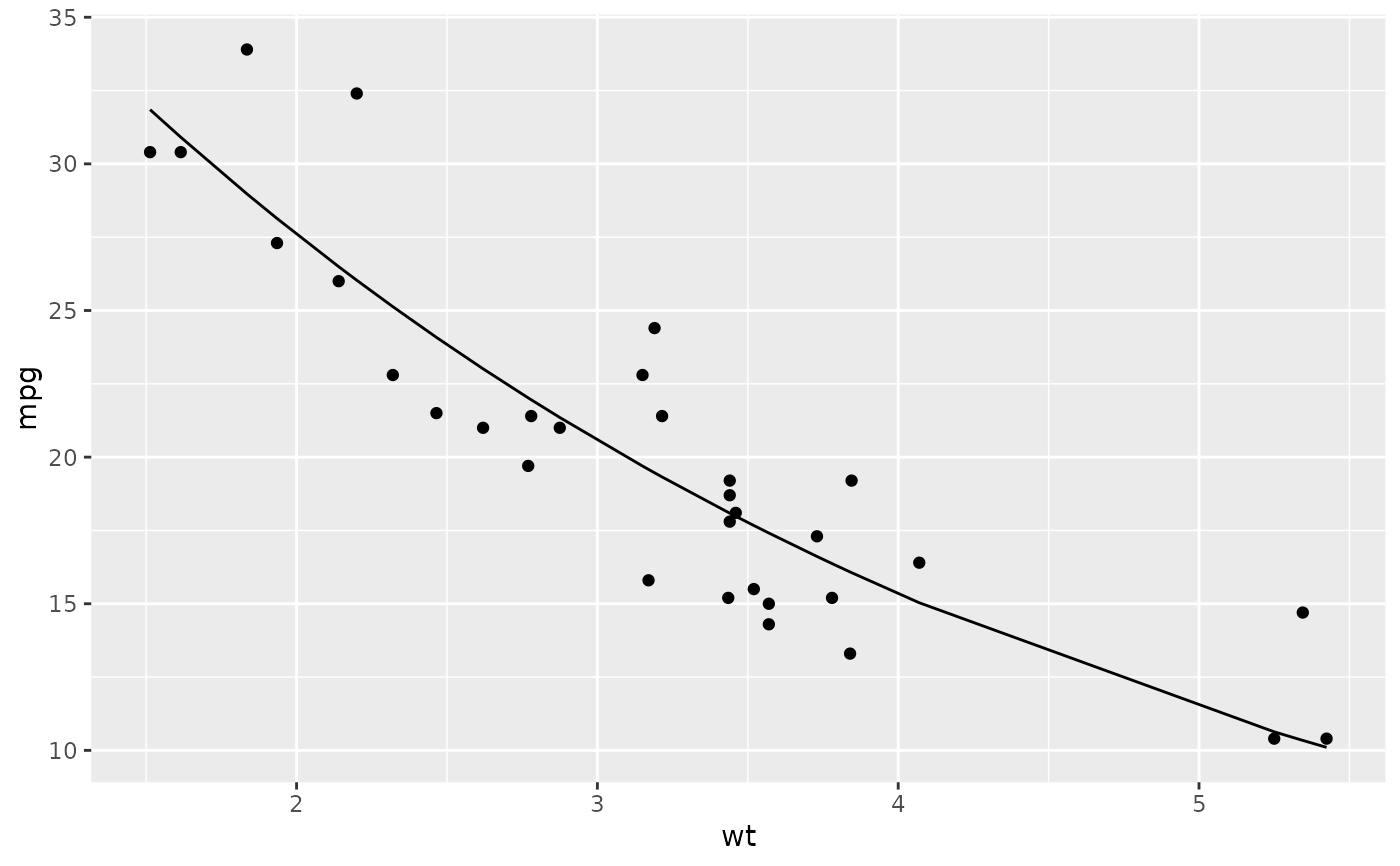
library(ggplot2)
ggplot(augment(n), aes(wt, mpg)) +
geom_point() +
geom_line(aes(y = .fitted))
 newdata <- head(mtcars)
newdata$wt <- newdata$wt + 1
augment(n, newdata = newdata)
#> # A tibble: 6 × 13
#> .rownames mpg cyl disp hp drat wt qsec vs am gear carb
#> <chr> <dbl> <dbl> <dbl> <dbl> <dbl> <dbl> <dbl> <dbl> <dbl> <dbl> <dbl>
#> 1 Mazda RX4 21 6 160 110 3.9 3.62 16.5 0 1 4 4
#> 2 Mazda RX4 W… 21 6 160 110 3.9 3.88 17.0 0 1 4 4
#> 3 Datsun 710 22.8 4 108 93 3.85 3.32 18.6 1 1 4 1
#> 4 Hornet 4 Dr… 21.4 6 258 110 3.08 4.22 19.4 1 0 3 1
#> 5 Hornet Spor… 18.7 8 360 175 3.15 4.44 17.0 0 0 3 2
#> 6 Valiant 18.1 6 225 105 2.76 4.46 20.2 1 0 3 1
#> # … with 1 more variable: .fitted <dbl>
newdata <- head(mtcars)
newdata$wt <- newdata$wt + 1
augment(n, newdata = newdata)
#> # A tibble: 6 × 13
#> .rownames mpg cyl disp hp drat wt qsec vs am gear carb
#> <chr> <dbl> <dbl> <dbl> <dbl> <dbl> <dbl> <dbl> <dbl> <dbl> <dbl> <dbl>
#> 1 Mazda RX4 21 6 160 110 3.9 3.62 16.5 0 1 4 4
#> 2 Mazda RX4 W… 21 6 160 110 3.9 3.88 17.0 0 1 4 4
#> 3 Datsun 710 22.8 4 108 93 3.85 3.32 18.6 1 1 4 1
#> 4 Hornet 4 Dr… 21.4 6 258 110 3.08 4.22 19.4 1 0 3 1
#> 5 Hornet Spor… 18.7 8 360 175 3.15 4.44 17.0 0 0 3 2
#> 6 Valiant 18.1 6 225 105 2.76 4.46 20.2 1 0 3 1
#> # … with 1 more variable: .fitted <dbl>