Glance accepts a model object and returns a tibble::tibble()
with exactly one row of model summaries. The summaries are typically
goodness of fit measures, p-values for hypothesis tests on residuals,
or model convergence information.
Glance never returns information from the original call to the modeling function. This includes the name of the modeling function or any arguments passed to the modeling function.
Glance does not calculate summary measures. Rather, it farms out these
computations to appropriate methods and gathers the results together.
Sometimes a goodness of fit measure will be undefined. In these cases
the measure will be reported as NA.
Glance returns the same number of columns regardless of whether the
model matrix is rank-deficient or not. If so, entries in columns
that no longer have a well-defined value are filled in with an NA
of the appropriate type.
# S3 method for nls
glance(x, ...)
Arguments
- x
An
nlsobject returned fromstats::nls().- ...
Additional arguments. Not used. Needed to match generic signature only. Cautionary note: Misspelled arguments will be absorbed in
..., where they will be ignored. If the misspelled argument has a default value, the default value will be used. For example, if you passconf.lvel = 0.9, all computation will proceed usingconf.level = 0.95. Additionally, if you passnewdata = my_tibbleto anaugment()method that does not accept anewdataargument, it will use the default value for thedataargument.
See also
Other nls tidiers:
augment.nls(),
tidy.nls()
Value
A tibble::tibble() with exactly one row and columns:
- AIC
Akaike's Information Criterion for the model.
- BIC
Bayesian Information Criterion for the model.
- deviance
Deviance of the model.
- df.residual
Residual degrees of freedom.
- finTol
The achieved convergence tolerance.
- isConv
Whether the fit successfully converged.
- logLik
The log-likelihood of the model. [stats::logLik()] may be a useful reference.
- nobs
Number of observations used.
- sigma
Estimated standard error of the residuals.
Examples
# fit model
n <- nls(mpg ~ k * e^wt, data = mtcars, start = list(k = 1, e = 2))
# summarize model fit with tidiers + visualization
tidy(n)
#> # A tibble: 2 × 5
#> term estimate std.error statistic p.value
#> <chr> <dbl> <dbl> <dbl> <dbl>
#> 1 k 49.7 3.79 13.1 5.96e-14
#> 2 e 0.746 0.0199 37.5 8.86e-27
augment(n)
#> # A tibble: 32 × 4
#> mpg wt .fitted .resid
#> <dbl> <dbl> <dbl> <dbl>
#> 1 21 2.62 23.0 -2.01
#> 2 21 2.88 21.4 -0.352
#> 3 22.8 2.32 25.1 -2.33
#> 4 21.4 3.22 19.3 2.08
#> 5 18.7 3.44 18.1 0.611
#> 6 18.1 3.46 18.0 0.117
#> 7 14.3 3.57 17.4 -3.11
#> 8 24.4 3.19 19.5 4.93
#> 9 22.8 3.15 19.7 3.10
#> 10 19.2 3.44 18.1 1.11
#> # … with 22 more rows
glance(n)
#> # A tibble: 1 × 9
#> sigma isConv finTol logLik AIC BIC deviance df.residual nobs
#> <dbl> <lgl> <dbl> <dbl> <dbl> <dbl> <dbl> <int> <int>
#> 1 2.67 TRUE 0.00000204 -75.8 158. 162. 214. 30 32
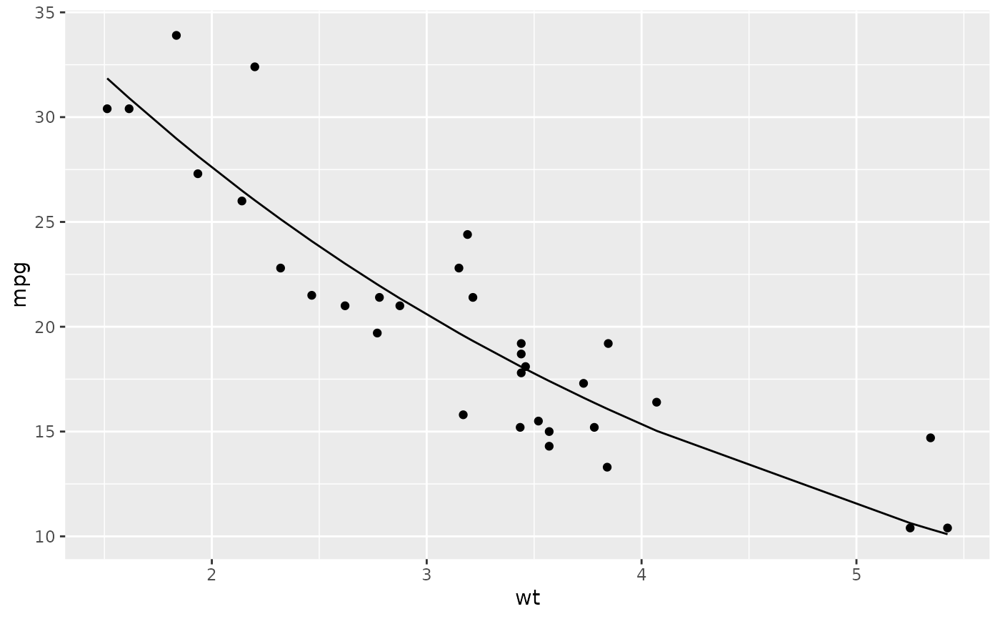
library(ggplot2)
ggplot(augment(n), aes(wt, mpg)) +
geom_point() +
geom_line(aes(y = .fitted))
 newdata <- head(mtcars)
newdata$wt <- newdata$wt + 1
augment(n, newdata = newdata)
#> # A tibble: 6 × 13
#> .rownames mpg cyl disp hp drat wt qsec vs am gear carb
#> <chr> <dbl> <dbl> <dbl> <dbl> <dbl> <dbl> <dbl> <dbl> <dbl> <dbl> <dbl>
#> 1 Mazda RX4 21 6 160 110 3.9 3.62 16.5 0 1 4 4
#> 2 Mazda RX4 W… 21 6 160 110 3.9 3.88 17.0 0 1 4 4
#> 3 Datsun 710 22.8 4 108 93 3.85 3.32 18.6 1 1 4 1
#> 4 Hornet 4 Dr… 21.4 6 258 110 3.08 4.22 19.4 1 0 3 1
#> 5 Hornet Spor… 18.7 8 360 175 3.15 4.44 17.0 0 0 3 2
#> 6 Valiant 18.1 6 225 105 2.76 4.46 20.2 1 0 3 1
#> # … with 1 more variable: .fitted <dbl>
newdata <- head(mtcars)
newdata$wt <- newdata$wt + 1
augment(n, newdata = newdata)
#> # A tibble: 6 × 13
#> .rownames mpg cyl disp hp drat wt qsec vs am gear carb
#> <chr> <dbl> <dbl> <dbl> <dbl> <dbl> <dbl> <dbl> <dbl> <dbl> <dbl> <dbl>
#> 1 Mazda RX4 21 6 160 110 3.9 3.62 16.5 0 1 4 4
#> 2 Mazda RX4 W… 21 6 160 110 3.9 3.88 17.0 0 1 4 4
#> 3 Datsun 710 22.8 4 108 93 3.85 3.32 18.6 1 1 4 1
#> 4 Hornet 4 Dr… 21.4 6 258 110 3.08 4.22 19.4 1 0 3 1
#> 5 Hornet Spor… 18.7 8 360 175 3.15 4.44 17.0 0 0 3 2
#> 6 Valiant 18.1 6 225 105 2.76 4.46 20.2 1 0 3 1
#> # … with 1 more variable: .fitted <dbl>