Tidy summarizes information about the components of a model. A model component might be a single term in a regression, a single hypothesis, a cluster, or a class. Exactly what tidy considers to be a model component varies across models but is usually self-evident. If a model has several distinct types of components, you will need to specify which components to return.
# S3 method for lm
tidy(x, conf.int = FALSE, conf.level = 0.95, ...)
Arguments
- x
An
lmobject created bystats::lm().- conf.int
Logical indicating whether or not to include a confidence interval in the tidied output. Defaults to
FALSE.- conf.level
The confidence level to use for the confidence interval if
conf.int = TRUE. Must be strictly greater than 0 and less than 1. Defaults to 0.95, which corresponds to a 95 percent confidence interval.- ...
Additional arguments. Not used. Needed to match generic signature only. Cautionary note: Misspelled arguments will be absorbed in
..., where they will be ignored. If the misspelled argument has a default value, the default value will be used. For example, if you passconf.lvel = 0.9, all computation will proceed usingconf.level = 0.95. Additionally, if you passnewdata = my_tibbleto anaugment()method that does not accept anewdataargument, it will use the default value for thedataargument.
Details
If the linear model is an mlm object (multiple linear model),
there is an additional column response. See tidy.mlm().
See also
Other lm tidiers:
augment.glm(),
augment.lm(),
glance.glm(),
glance.lm(),
glance.summary.lm(),
glance.svyglm(),
tidy.glm(),
tidy.lm.beta(),
tidy.mlm(),
tidy.summary.lm()
Value
A tibble::tibble() with columns:
- conf.high
Upper bound on the confidence interval for the estimate.
- conf.low
Lower bound on the confidence interval for the estimate.
- estimate
The estimated value of the regression term.
- p.value
The two-sided p-value associated with the observed statistic.
- statistic
The value of a T-statistic to use in a hypothesis that the regression term is non-zero.
- std.error
The standard error of the regression term.
- term
The name of the regression term.
Examples
library(ggplot2)
library(dplyr)
mod <- lm(mpg ~ wt + qsec, data = mtcars)
tidy(mod)
#> # A tibble: 3 × 5
#> term estimate std.error statistic p.value
#> <chr> <dbl> <dbl> <dbl> <dbl>
#> 1 (Intercept) 19.7 5.25 3.76 7.65e- 4
#> 2 wt -5.05 0.484 -10.4 2.52e-11
#> 3 qsec 0.929 0.265 3.51 1.50e- 3
glance(mod)
#> # A tibble: 1 × 12
#> r.squared adj.r.squared sigma statistic p.value df logLik AIC BIC
#> <dbl> <dbl> <dbl> <dbl> <dbl> <dbl> <dbl> <dbl> <dbl>
#> 1 0.826 0.814 2.60 69.0 9.39e-12 2 -74.4 157. 163.
#> # … with 3 more variables: deviance <dbl>, df.residual <int>, nobs <int>
# coefficient plot
d <- tidy(mod, conf.int = TRUE)
ggplot(d, aes(estimate, term, xmin = conf.low, xmax = conf.high, height = 0)) +
geom_point() +
geom_vline(xintercept = 0, lty = 4) +
geom_errorbarh()
 # aside: There are tidy() and glance() methods for lm.summary objects too.
# this can be useful when you want to conserve memory by converting large lm
# objects into their leaner summary.lm equivalents.
s <- summary(mod)
tidy(s, conf.int = TRUE)
#> # A tibble: 3 × 7
#> term estimate std.error statistic p.value conf.low conf.high
#> <chr> <dbl> <dbl> <dbl> <dbl> <dbl> <dbl>
#> 1 (Intercept) 19.7 5.25 3.76 7.65e- 4 9.00 30.5
#> 2 wt -5.05 0.484 -10.4 2.52e-11 -6.04 -4.06
#> 3 qsec 0.929 0.265 3.51 1.50e- 3 0.387 1.47
glance(s)
#> # A tibble: 1 × 8
#> r.squared adj.r.squared sigma statistic p.value df df.residual nobs
#> <dbl> <dbl> <dbl> <dbl> <dbl> <dbl> <int> <dbl>
#> 1 0.826 0.814 2.60 69.0 9.39e-12 2 29 32
augment(mod)
#> # A tibble: 32 × 10
#> .rownames mpg wt qsec .fitted .resid .hat .sigma .cooksd .std.resid
#> <chr> <dbl> <dbl> <dbl> <dbl> <dbl> <dbl> <dbl> <dbl> <dbl>
#> 1 Mazda RX4 21 2.62 16.5 21.8 -0.815 0.0693 2.64 2.63e-3 -0.325
#> 2 Mazda RX4… 21 2.88 17.0 21.0 -0.0482 0.0444 2.64 5.59e-6 -0.0190
#> 3 Datsun 710 22.8 2.32 18.6 25.3 -2.53 0.0607 2.60 2.17e-2 -1.00
#> 4 Hornet 4 … 21.4 3.22 19.4 21.6 -0.181 0.0576 2.64 1.05e-4 -0.0716
#> 5 Hornet Sp… 18.7 3.44 17.0 18.2 0.504 0.0389 2.64 5.29e-4 0.198
#> 6 Valiant 18.1 3.46 20.2 21.1 -2.97 0.0957 2.58 5.10e-2 -1.20
#> 7 Duster 360 14.3 3.57 15.8 16.4 -2.14 0.0729 2.61 1.93e-2 -0.857
#> 8 Merc 240D 24.4 3.19 20 22.2 2.17 0.0791 2.61 2.18e-2 0.872
#> 9 Merc 230 22.8 3.15 22.9 25.1 -2.32 0.295 2.59 1.59e-1 -1.07
#> 10 Merc 280 19.2 3.44 18.3 19.4 -0.185 0.0358 2.64 6.55e-5 -0.0728
#> # … with 22 more rows
augment(mod, mtcars, interval = "confidence")
#> # A tibble: 32 × 20
#> .rownames mpg cyl disp hp drat wt qsec vs am gear carb
#> <chr> <dbl> <dbl> <dbl> <dbl> <dbl> <dbl> <dbl> <dbl> <dbl> <dbl> <dbl>
#> 1 Mazda RX4 21 6 160 110 3.9 2.62 16.5 0 1 4 4
#> 2 Mazda RX4 … 21 6 160 110 3.9 2.88 17.0 0 1 4 4
#> 3 Datsun 710 22.8 4 108 93 3.85 2.32 18.6 1 1 4 1
#> 4 Hornet 4 D… 21.4 6 258 110 3.08 3.22 19.4 1 0 3 1
#> 5 Hornet Spo… 18.7 8 360 175 3.15 3.44 17.0 0 0 3 2
#> 6 Valiant 18.1 6 225 105 2.76 3.46 20.2 1 0 3 1
#> 7 Duster 360 14.3 8 360 245 3.21 3.57 15.8 0 0 3 4
#> 8 Merc 240D 24.4 4 147. 62 3.69 3.19 20 1 0 4 2
#> 9 Merc 230 22.8 4 141. 95 3.92 3.15 22.9 1 0 4 2
#> 10 Merc 280 19.2 6 168. 123 3.92 3.44 18.3 1 0 4 4
#> # … with 22 more rows, and 8 more variables: .fitted <dbl>, .lower <dbl>,
#> # .upper <dbl>, .resid <dbl>, .hat <dbl>, .sigma <dbl>, .cooksd <dbl>,
#> # .std.resid <dbl>
# predict on new data
newdata <- mtcars %>%
head(6) %>%
mutate(wt = wt + 1)
augment(mod, newdata = newdata)
#> # A tibble: 6 × 14
#> .rownames mpg cyl disp hp drat wt qsec vs am gear carb
#> <chr> <dbl> <dbl> <dbl> <dbl> <dbl> <dbl> <dbl> <dbl> <dbl> <dbl> <dbl>
#> 1 Mazda RX4 21 6 160 110 3.9 3.62 16.5 0 1 4 4
#> 2 Mazda RX4 W… 21 6 160 110 3.9 3.88 17.0 0 1 4 4
#> 3 Datsun 710 22.8 4 108 93 3.85 3.32 18.6 1 1 4 1
#> 4 Hornet 4 Dr… 21.4 6 258 110 3.08 4.22 19.4 1 0 3 1
#> 5 Hornet Spor… 18.7 8 360 175 3.15 4.44 17.0 0 0 3 2
#> 6 Valiant 18.1 6 225 105 2.76 4.46 20.2 1 0 3 1
#> # … with 2 more variables: .fitted <dbl>, .resid <dbl>
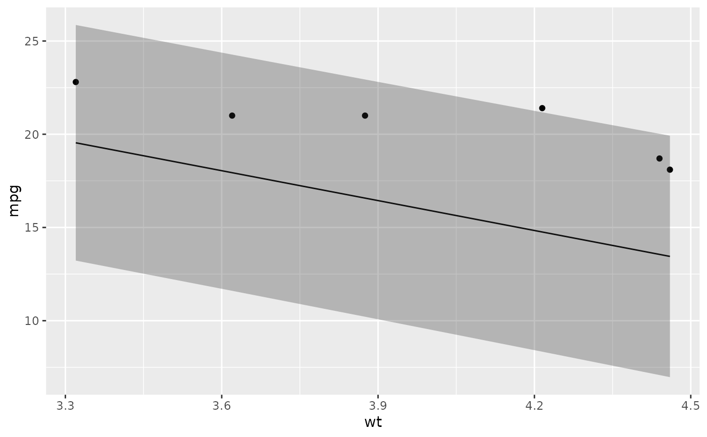
# ggplot2 example where we also construct 95% prediction interval
# simpler bivariate model since we're plotting in 2D
mod2 <- lm(mpg ~ wt, data = mtcars)
au <- augment(mod2, newdata = newdata, interval = "prediction")
ggplot(au, aes(wt, mpg)) +
geom_point() +
geom_line(aes(y = .fitted)) +
geom_ribbon(aes(ymin = .lower, ymax = .upper), col = NA, alpha = 0.3)
# aside: There are tidy() and glance() methods for lm.summary objects too.
# this can be useful when you want to conserve memory by converting large lm
# objects into their leaner summary.lm equivalents.
s <- summary(mod)
tidy(s, conf.int = TRUE)
#> # A tibble: 3 × 7
#> term estimate std.error statistic p.value conf.low conf.high
#> <chr> <dbl> <dbl> <dbl> <dbl> <dbl> <dbl>
#> 1 (Intercept) 19.7 5.25 3.76 7.65e- 4 9.00 30.5
#> 2 wt -5.05 0.484 -10.4 2.52e-11 -6.04 -4.06
#> 3 qsec 0.929 0.265 3.51 1.50e- 3 0.387 1.47
glance(s)
#> # A tibble: 1 × 8
#> r.squared adj.r.squared sigma statistic p.value df df.residual nobs
#> <dbl> <dbl> <dbl> <dbl> <dbl> <dbl> <int> <dbl>
#> 1 0.826 0.814 2.60 69.0 9.39e-12 2 29 32
augment(mod)
#> # A tibble: 32 × 10
#> .rownames mpg wt qsec .fitted .resid .hat .sigma .cooksd .std.resid
#> <chr> <dbl> <dbl> <dbl> <dbl> <dbl> <dbl> <dbl> <dbl> <dbl>
#> 1 Mazda RX4 21 2.62 16.5 21.8 -0.815 0.0693 2.64 2.63e-3 -0.325
#> 2 Mazda RX4… 21 2.88 17.0 21.0 -0.0482 0.0444 2.64 5.59e-6 -0.0190
#> 3 Datsun 710 22.8 2.32 18.6 25.3 -2.53 0.0607 2.60 2.17e-2 -1.00
#> 4 Hornet 4 … 21.4 3.22 19.4 21.6 -0.181 0.0576 2.64 1.05e-4 -0.0716
#> 5 Hornet Sp… 18.7 3.44 17.0 18.2 0.504 0.0389 2.64 5.29e-4 0.198
#> 6 Valiant 18.1 3.46 20.2 21.1 -2.97 0.0957 2.58 5.10e-2 -1.20
#> 7 Duster 360 14.3 3.57 15.8 16.4 -2.14 0.0729 2.61 1.93e-2 -0.857
#> 8 Merc 240D 24.4 3.19 20 22.2 2.17 0.0791 2.61 2.18e-2 0.872
#> 9 Merc 230 22.8 3.15 22.9 25.1 -2.32 0.295 2.59 1.59e-1 -1.07
#> 10 Merc 280 19.2 3.44 18.3 19.4 -0.185 0.0358 2.64 6.55e-5 -0.0728
#> # … with 22 more rows
augment(mod, mtcars, interval = "confidence")
#> # A tibble: 32 × 20
#> .rownames mpg cyl disp hp drat wt qsec vs am gear carb
#> <chr> <dbl> <dbl> <dbl> <dbl> <dbl> <dbl> <dbl> <dbl> <dbl> <dbl> <dbl>
#> 1 Mazda RX4 21 6 160 110 3.9 2.62 16.5 0 1 4 4
#> 2 Mazda RX4 … 21 6 160 110 3.9 2.88 17.0 0 1 4 4
#> 3 Datsun 710 22.8 4 108 93 3.85 2.32 18.6 1 1 4 1
#> 4 Hornet 4 D… 21.4 6 258 110 3.08 3.22 19.4 1 0 3 1
#> 5 Hornet Spo… 18.7 8 360 175 3.15 3.44 17.0 0 0 3 2
#> 6 Valiant 18.1 6 225 105 2.76 3.46 20.2 1 0 3 1
#> 7 Duster 360 14.3 8 360 245 3.21 3.57 15.8 0 0 3 4
#> 8 Merc 240D 24.4 4 147. 62 3.69 3.19 20 1 0 4 2
#> 9 Merc 230 22.8 4 141. 95 3.92 3.15 22.9 1 0 4 2
#> 10 Merc 280 19.2 6 168. 123 3.92 3.44 18.3 1 0 4 4
#> # … with 22 more rows, and 8 more variables: .fitted <dbl>, .lower <dbl>,
#> # .upper <dbl>, .resid <dbl>, .hat <dbl>, .sigma <dbl>, .cooksd <dbl>,
#> # .std.resid <dbl>
# predict on new data
newdata <- mtcars %>%
head(6) %>%
mutate(wt = wt + 1)
augment(mod, newdata = newdata)
#> # A tibble: 6 × 14
#> .rownames mpg cyl disp hp drat wt qsec vs am gear carb
#> <chr> <dbl> <dbl> <dbl> <dbl> <dbl> <dbl> <dbl> <dbl> <dbl> <dbl> <dbl>
#> 1 Mazda RX4 21 6 160 110 3.9 3.62 16.5 0 1 4 4
#> 2 Mazda RX4 W… 21 6 160 110 3.9 3.88 17.0 0 1 4 4
#> 3 Datsun 710 22.8 4 108 93 3.85 3.32 18.6 1 1 4 1
#> 4 Hornet 4 Dr… 21.4 6 258 110 3.08 4.22 19.4 1 0 3 1
#> 5 Hornet Spor… 18.7 8 360 175 3.15 4.44 17.0 0 0 3 2
#> 6 Valiant 18.1 6 225 105 2.76 4.46 20.2 1 0 3 1
#> # … with 2 more variables: .fitted <dbl>, .resid <dbl>
# ggplot2 example where we also construct 95% prediction interval
# simpler bivariate model since we're plotting in 2D
mod2 <- lm(mpg ~ wt, data = mtcars)
au <- augment(mod2, newdata = newdata, interval = "prediction")
ggplot(au, aes(wt, mpg)) +
geom_point() +
geom_line(aes(y = .fitted)) +
geom_ribbon(aes(ymin = .lower, ymax = .upper), col = NA, alpha = 0.3)
 # predict on new data without outcome variable. Output does not include .resid
newdata <- newdata %>%
select(-mpg)
augment(mod, newdata = newdata)
#> Warning: 'newdata' had 6 rows but variables found have 234 rows
#> # A tibble: 6 × 12
#> .rownames cyl disp hp drat wt qsec vs am gear carb .fitted
#> <chr> <dbl> <dbl> <dbl> <dbl> <dbl> <dbl> <dbl> <dbl> <dbl> <dbl> <dbl>
#> 1 Mazda RX4 6 160 110 3.9 3.62 16.5 0 1 4 4 16.8
#> 2 Mazda RX4… 6 160 110 3.9 3.88 17.0 0 1 4 4 16.0
#> 3 Datsun 710 4 108 93 3.85 3.32 18.6 1 1 4 1 20.3
#> 4 Hornet 4 … 6 258 110 3.08 4.22 19.4 1 0 3 1 16.5
#> 5 Hornet Sp… 8 360 175 3.15 4.44 17.0 0 0 3 2 13.1
#> 6 Valiant 6 225 105 2.76 4.46 20.2 1 0 3 1 16.0
au <- augment(mod, data = mtcars)
ggplot(au, aes(.hat, .std.resid)) +
geom_vline(size = 2, colour = "white", xintercept = 0) +
geom_hline(size = 2, colour = "white", yintercept = 0) +
geom_point() +
geom_smooth(se = FALSE)
#> `geom_smooth()` using method = 'loess' and formula 'y ~ x'
# predict on new data without outcome variable. Output does not include .resid
newdata <- newdata %>%
select(-mpg)
augment(mod, newdata = newdata)
#> Warning: 'newdata' had 6 rows but variables found have 234 rows
#> # A tibble: 6 × 12
#> .rownames cyl disp hp drat wt qsec vs am gear carb .fitted
#> <chr> <dbl> <dbl> <dbl> <dbl> <dbl> <dbl> <dbl> <dbl> <dbl> <dbl> <dbl>
#> 1 Mazda RX4 6 160 110 3.9 3.62 16.5 0 1 4 4 16.8
#> 2 Mazda RX4… 6 160 110 3.9 3.88 17.0 0 1 4 4 16.0
#> 3 Datsun 710 4 108 93 3.85 3.32 18.6 1 1 4 1 20.3
#> 4 Hornet 4 … 6 258 110 3.08 4.22 19.4 1 0 3 1 16.5
#> 5 Hornet Sp… 8 360 175 3.15 4.44 17.0 0 0 3 2 13.1
#> 6 Valiant 6 225 105 2.76 4.46 20.2 1 0 3 1 16.0
au <- augment(mod, data = mtcars)
ggplot(au, aes(.hat, .std.resid)) +
geom_vline(size = 2, colour = "white", xintercept = 0) +
geom_hline(size = 2, colour = "white", yintercept = 0) +
geom_point() +
geom_smooth(se = FALSE)
#> `geom_smooth()` using method = 'loess' and formula 'y ~ x'
 plot(mod, which = 6)
 ggplot(au, aes(.hat, .cooksd)) +
geom_vline(xintercept = 0, colour = NA) +
geom_abline(slope = seq(0, 3, by = 0.5), colour = "white") +
geom_smooth(se = FALSE) +
geom_point()
#> `geom_smooth()` using method = 'loess' and formula 'y ~ x'
ggplot(au, aes(.hat, .cooksd)) +
geom_vline(xintercept = 0, colour = NA) +
geom_abline(slope = seq(0, 3, by = 0.5), colour = "white") +
geom_smooth(se = FALSE) +
geom_point()
#> `geom_smooth()` using method = 'loess' and formula 'y ~ x'
 # column-wise models
a <- matrix(rnorm(20), nrow = 10)
b <- a + rnorm(length(a))
result <- lm(b ~ a)
tidy(result)
#> # A tibble: 6 × 6
#> response term estimate std.error statistic p.value
#> <chr> <chr> <dbl> <dbl> <dbl> <dbl>
#> 1 Y1 (Intercept) 0.120 0.460 0.260 0.802
#> 2 Y1 a1 1.40 0.400 3.51 0.00987
#> 3 Y1 a2 0.00979 0.337 0.0291 0.978
#> 4 Y2 (Intercept) -0.300 0.320 -0.940 0.379
#> 5 Y2 a1 0.160 0.278 0.578 0.582
#> 6 Y2 a2 0.913 0.234 3.90 0.00589
# column-wise models
a <- matrix(rnorm(20), nrow = 10)
b <- a + rnorm(length(a))
result <- lm(b ~ a)
tidy(result)
#> # A tibble: 6 × 6
#> response term estimate std.error statistic p.value
#> <chr> <chr> <dbl> <dbl> <dbl> <dbl>
#> 1 Y1 (Intercept) 0.120 0.460 0.260 0.802
#> 2 Y1 a1 1.40 0.400 3.51 0.00987
#> 3 Y1 a2 0.00979 0.337 0.0291 0.978
#> 4 Y2 (Intercept) -0.300 0.320 -0.940 0.379
#> 5 Y2 a1 0.160 0.278 0.578 0.582
#> 6 Y2 a2 0.913 0.234 3.90 0.00589