Tidy summarizes information about the components of a model. A model component might be a single term in a regression, a single hypothesis, a cluster, or a class. Exactly what tidy considers to be a model component varies across models but is usually self-evident. If a model has several distinct types of components, you will need to specify which components to return.
# S3 method for rcorr
tidy(x, diagonal = FALSE, ...)
Arguments
- x
An
rcorrobject returned fromHmisc::rcorr().- diagonal
Logical indicating whether or not to include diagonal elements of the correlation matrix, or the correlation of a column with itself. For the elements,
estimateis always 1 andp.valueis alwaysNA. Defaults toFALSE.- ...
Additional arguments. Not used. Needed to match generic signature only. Cautionary note: Misspelled arguments will be absorbed in
..., where they will be ignored. If the misspelled argument has a default value, the default value will be used. For example, if you passconf.lvel = 0.9, all computation will proceed usingconf.level = 0.95. Additionally, if you passnewdata = my_tibbleto anaugment()method that does not accept anewdataargument, it will use the default value for thedataargument.
Details
Suppose the original data has columns A and B. In the correlation
matrix from rcorr there may be entries for both the cor(A, B) and
cor(B, A). Only one of these pairs will ever be present in the tidy
output.
See also
Value
A tibble::tibble() with columns:
- column1
Name or index of the first column being described.
- column2
Name or index of the second column being described.
- estimate
The estimated value of the regression term.
- p.value
The two-sided p-value associated with the observed statistic.
- n
Number of observations used to compute the correlation
Examples
# feel free to ignore the following line—it allows {broom} to supply
# examples without requiring the model-supplying package to be installed.
if (requireNamespace("Hmisc", quietly = TRUE)) {
# load libraries for models and data
library(Hmisc)
mat <- replicate(52, rnorm(100))
# add some NAs
mat[sample(length(mat), 2000)] <- NA
# also, column names
colnames(mat) <- c(LETTERS, letters)
# fit model
rc <- rcorr(mat)
# summarize model fit with tidiers + visualization
td <- tidy(rc)
td
library(ggplot2)
ggplot(td, aes(p.value)) +
geom_histogram(binwidth = .1)
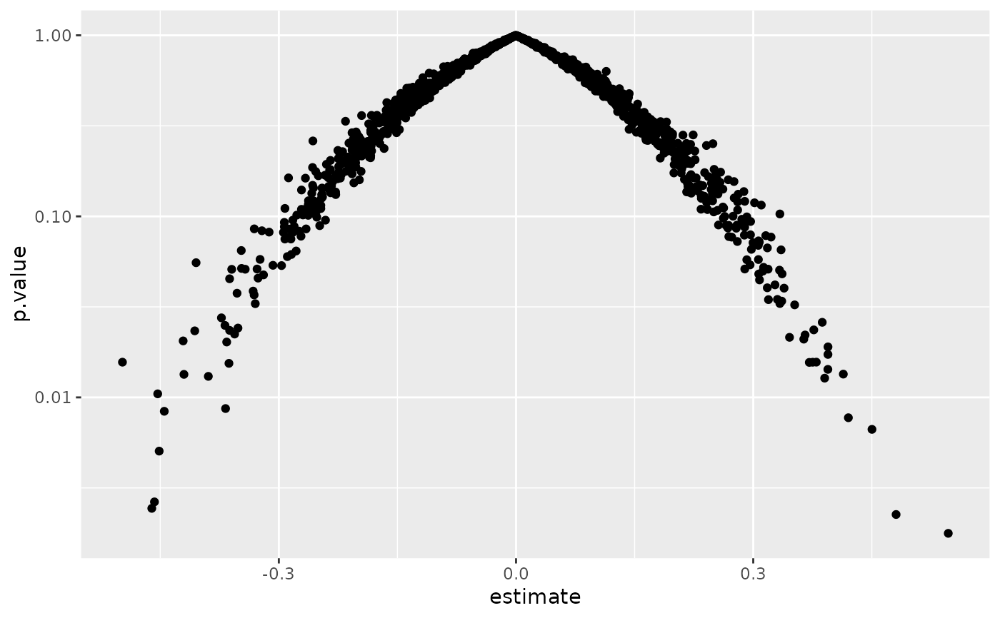
ggplot(td, aes(estimate, p.value)) +
geom_point() +
scale_y_log10()
}
#> Loading required package: Formula
#>
#> Attaching package: ‘Hmisc’
#> The following object is masked from ‘package:psych’:
#>
#> describe
#> The following object is masked from ‘package:network’:
#>
#> is.discrete
#> The following object is masked from ‘package:survey’:
#>
#> deff
#> The following object is masked from ‘package:quantreg’:
#>
#> latex
#> The following objects are masked from ‘package:dplyr’:
#>
#> src, summarize
#> The following objects are masked from ‘package:base’:
#>
#> format.pval, units