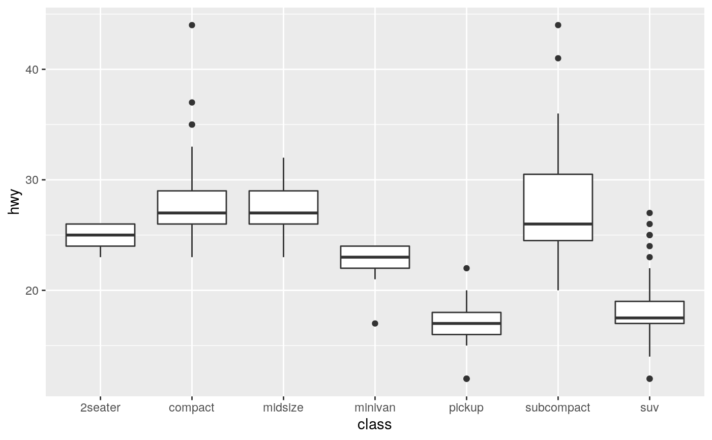
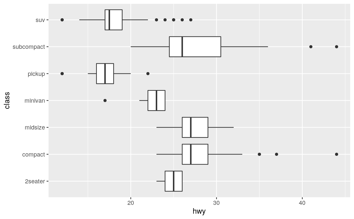
A box and whiskers plot (in the style of Tukey)

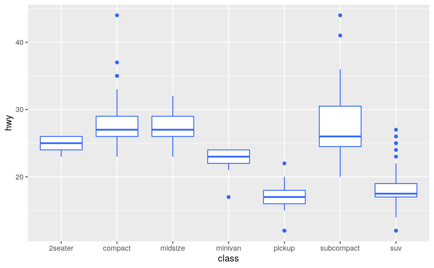
The boxplot compactly displays the distribution of a continuous variable. It visualises five summary statistics (the median, two hinges and two whiskers), and all "outlying" points individually.

geom_boxplot(mapping = NULL, data = NULL, stat = "boxplot",
  position = "dodge2", ..., outlier.colour = NULL,
  outlier.color = NULL, outlier.fill = NULL, outlier.shape = 19,
  outlier.size = 1.5, outlier.stroke = 0.5, outlier.alpha = NULL,
  notch = FALSE, notchwidth = 0.5, varwidth = FALSE, na.rm = FALSE,
  show.legend = NA, inherit.aes = TRUE)

stat_boxplot(mapping = NULL, data = NULL, geom = "boxplot",
  position = "dodge2", ..., coef = 1.5, na.rm = FALSE,
  show.legend = NA, inherit.aes = TRUE)

Arguments

mapping	Set of aesthetic mappings created by `aes()` or `aes_()`. If specified and `inherit.aes = TRUE` (the default), it is combined with the default mapping at the top level of the plot. You must supply `mapping` if there is no plot mapping.
data	The data to be displayed in this layer. There are three options: If `NULL`, the default, the data is inherited from the plot data as specified in the call to `ggplot()`. A `data.frame`, or other object, will override the plot data. All objects will be fortified to produce a data frame. See `fortify()` for which variables will be created. A `function` will be called with a single argument, the plot data. The return value must be a `data.frame`, and will be used as the layer data. A `function` can be created from a `formula` (e.g. `~ head(.x, 10)`).
position	Position adjustment, either as a string, or the result of a call to a position adjustment function.
...	Other arguments passed on to `layer()`. These are often aesthetics, used to set an aesthetic to a fixed value, like `colour = "red"` or `size = 3`. They may also be parameters to the paired geom/stat.
outlier.colour, outlier.color, outlier.fill, outlier.shape, outlier.size, outlier.stroke, outlier.alpha	Default aesthetics for outliers. Set to `NULL` to inherit from the aesthetics used for the box. In the unlikely event you specify both US and UK spellings of colour, the US spelling will take precedence. Sometimes it can be useful to hide the outliers, for example when overlaying the raw data points on top of the boxplot. Hiding the outliers can be achieved by setting `outlier.shape = NA`. Importantly, this does not remove the outliers, it only hides them, so the range calculated for the y-axis will be the same with outliers shown and outliers hidden.
notch	If `FALSE` (default) make a standard box plot. If `TRUE`, make a notched box plot. Notches are used to compare groups; if the notches of two boxes do not overlap, this suggests that the medians are significantly different.
notchwidth	For a notched box plot, width of the notch relative to the body (defaults to `notchwidth = 0.5`).
varwidth	If `FALSE` (default) make a standard box plot. If `TRUE`, boxes are drawn with widths proportional to the square-roots of the number of observations in the groups (possibly weighted, using the `weight` aesthetic).
na.rm	If `FALSE`, the default, missing values are removed with a warning. If `TRUE`, missing values are silently removed.
show.legend	logical. Should this layer be included in the legends? `NA`, the default, includes if any aesthetics are mapped. `FALSE` never includes, and `TRUE` always includes. It can also be a named logical vector to finely select the aesthetics to display.
inherit.aes	If `FALSE`, overrides the default aesthetics, rather than combining with them. This is most useful for helper functions that define both data and aesthetics and shouldn't inherit behaviour from the default plot specification, e.g. `borders()`.
geom, stat	Use to override the default connection between `geom_boxplot` and `stat_boxplot`.
coef	Length of the whiskers as multiple of IQR. Defaults to 1.5.

Summary statistics

The lower and upper hinges correspond to the first and third quartiles (the 25th and 75th percentiles). This differs slightly from the method used by the boxplot() function, and may be apparent with small samples. See boxplot.stats() for for more information on how hinge positions are calculated for boxplot().

The upper whisker extends from the hinge to the largest value no further than 1.5 * IQR from the hinge (where IQR is the inter-quartile range, or distance between the first and third quartiles). The lower whisker extends from the hinge to the smallest value at most 1.5 * IQR of the hinge. Data beyond the end of the whiskers are called "outlying" points and are plotted individually.

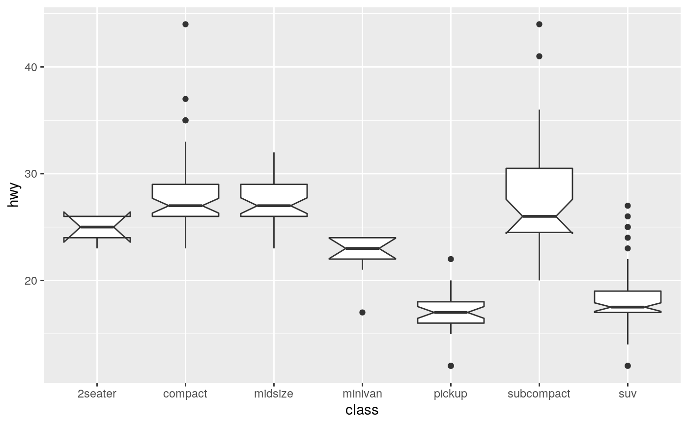
In a notched box plot, the notches extend 1.58 * IQR / sqrt(n). This gives a roughly 95% confidence interval for comparing medians. See McGill et al. (1978) for more details.

Aesthetics

geom_boxplot() understands the following aesthetics (required aesthetics are in bold):

x
lower
upper
middle
ymin
ymax
alpha
colour
fill
group
linetype
shape
size
weight

Learn more about setting these aesthetics in vignette("ggplot2-specs").

Computed variables

width: width of boxplot
ymin: lower whisker = smallest observation greater than or equal to lower hinge - 1.5 * IQR
lower: lower hinge, 25% quantile
notchlower: lower edge of notch = median - 1.58 * IQR / sqrt(n)
middle: median, 50% quantile
notchupper: upper edge of notch = median + 1.58 * IQR / sqrt(n)
upper: upper hinge, 75% quantile
ymax: upper whisker = largest observation less than or equal to upper hinge + 1.5 * IQR

References

McGill, R., Tukey, J. W. and Larsen, W. A. (1978) Variations of box plots. The American Statistician 32, 12-16.

Examples

p <- ggplot(mpg, aes(class, hwy))
p + geom_boxplot()
p + geom_boxplot() + coord_flip()

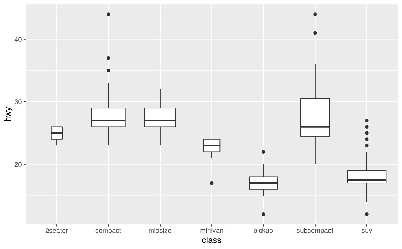
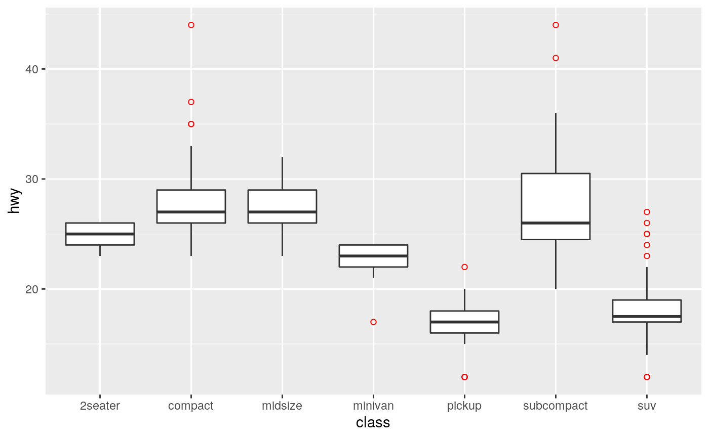
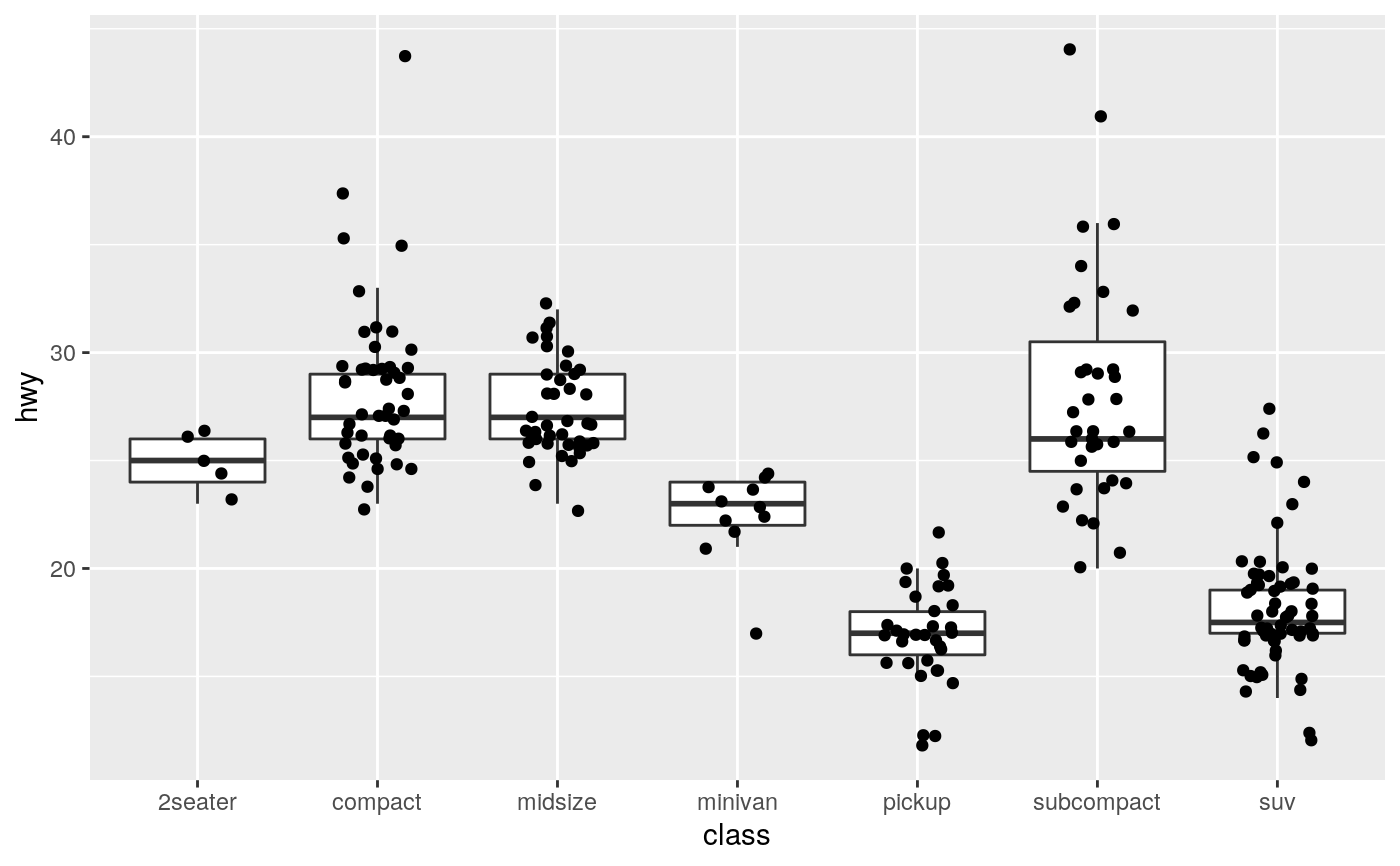
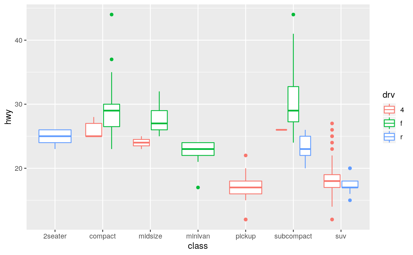
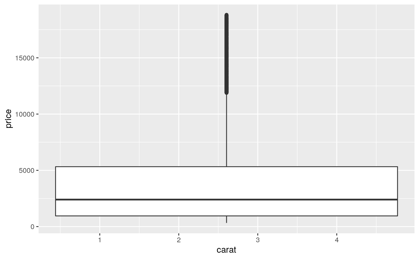
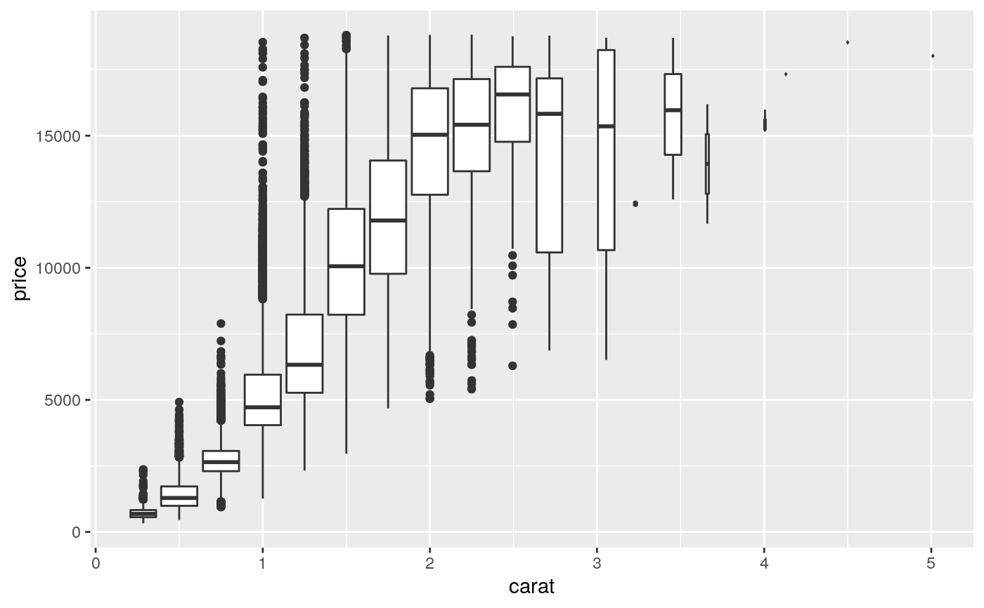
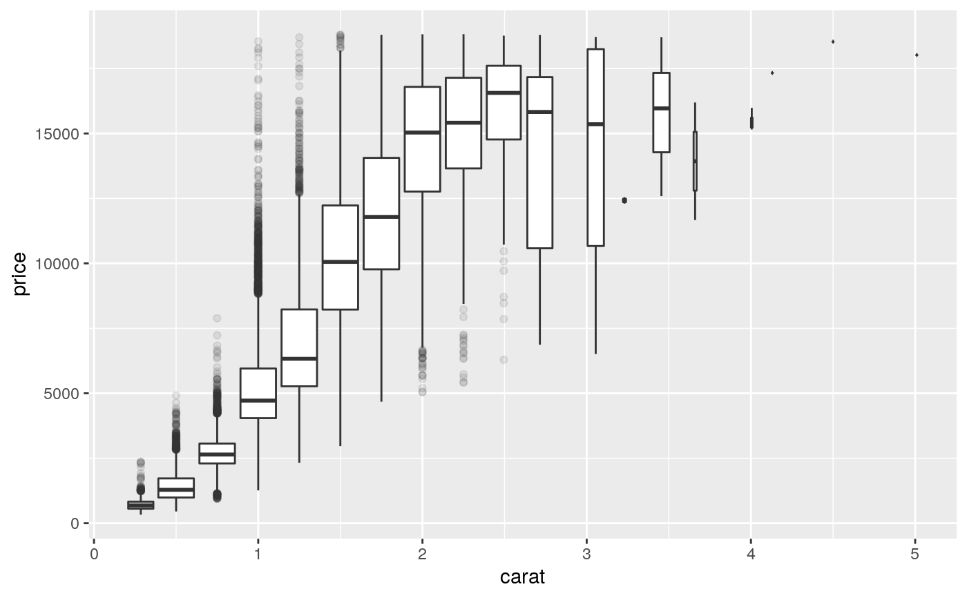
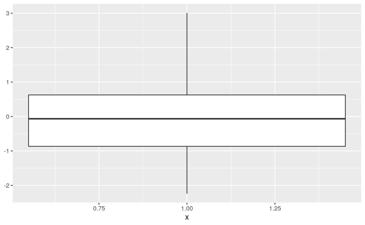
p + geom_boxplot(notch = TRUE)
#> notch went outside hinges. Try setting notch=FALSE.
#> notch went outside hinges. Try setting notch=FALSE.
p + geom_boxplot(varwidth = TRUE)
p + geom_boxplot(fill = "white", colour = "#3366FF")
# By default, outlier points match the colour of the box. Use
# outlier.colour to override
p + geom_boxplot(outlier.colour = "red", outlier.shape = 1)
# Remove outliers when overlaying boxplot with original data points
p + geom_boxplot(outlier.shape = NA) + geom_jitter(width = 0.2)

# Boxplots are automatically dodged when any aesthetic is a factor
p + geom_boxplot(aes(colour = drv))

# You can also use boxplots with continuous x, as long as you supply
# a grouping variable. cut_width is particularly useful
ggplot(diamonds, aes(carat, price)) +
  geom_boxplot()
#> Warning: Continuous x aesthetic -- did you forget aes(group=...)?
ggplot(diamonds, aes(carat, price)) +
  geom_boxplot(aes(group = cut_width(carat, 0.25)))
# Adjust the transparency of outliers using outlier.alpha
ggplot(diamonds, aes(carat, price)) +
  geom_boxplot(aes(group = cut_width(carat, 0.25)), outlier.alpha = 0.1)

# \donttest{
# It's possible to draw a boxplot with your own computations if you
# use stat = "identity":
y <- rnorm(100)
df <- data.frame(
  x = 1,
  y0 = min(y),
  y25 = quantile(y, 0.25),
  y50 = median(y),
  y75 = quantile(y, 0.75),
  y100 = max(y)
)
ggplot(df, aes(x)) +
  geom_boxplot(
   aes(ymin = y0, lower = y25, middle = y50, upper = y75, ymax = y100),
   stat = "identity"
 )
# }