Dot plot — geom_dotplot • ggplot2

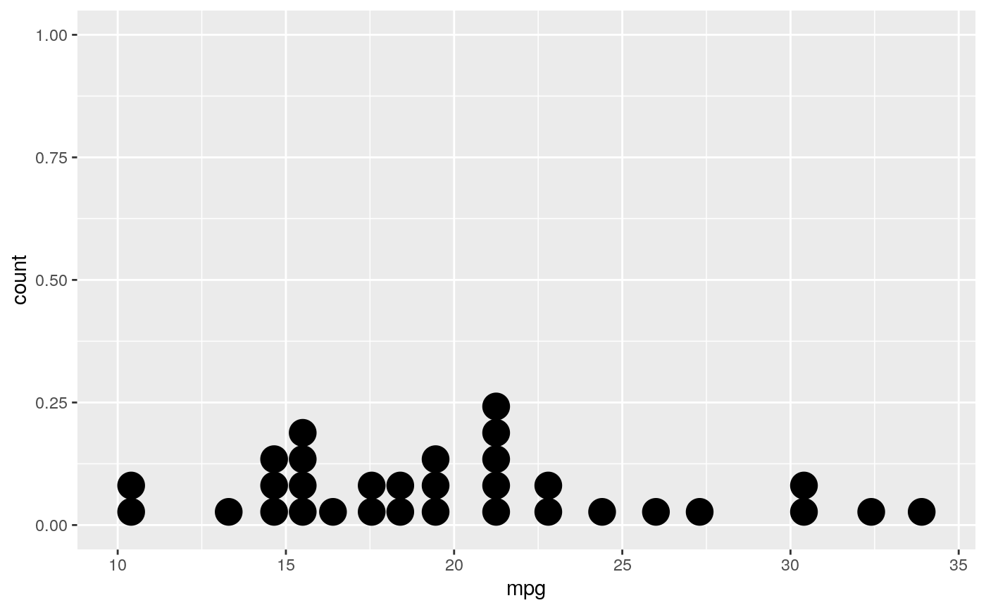
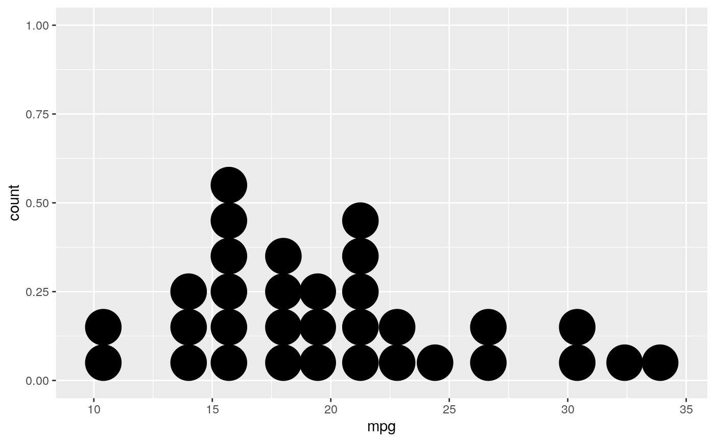
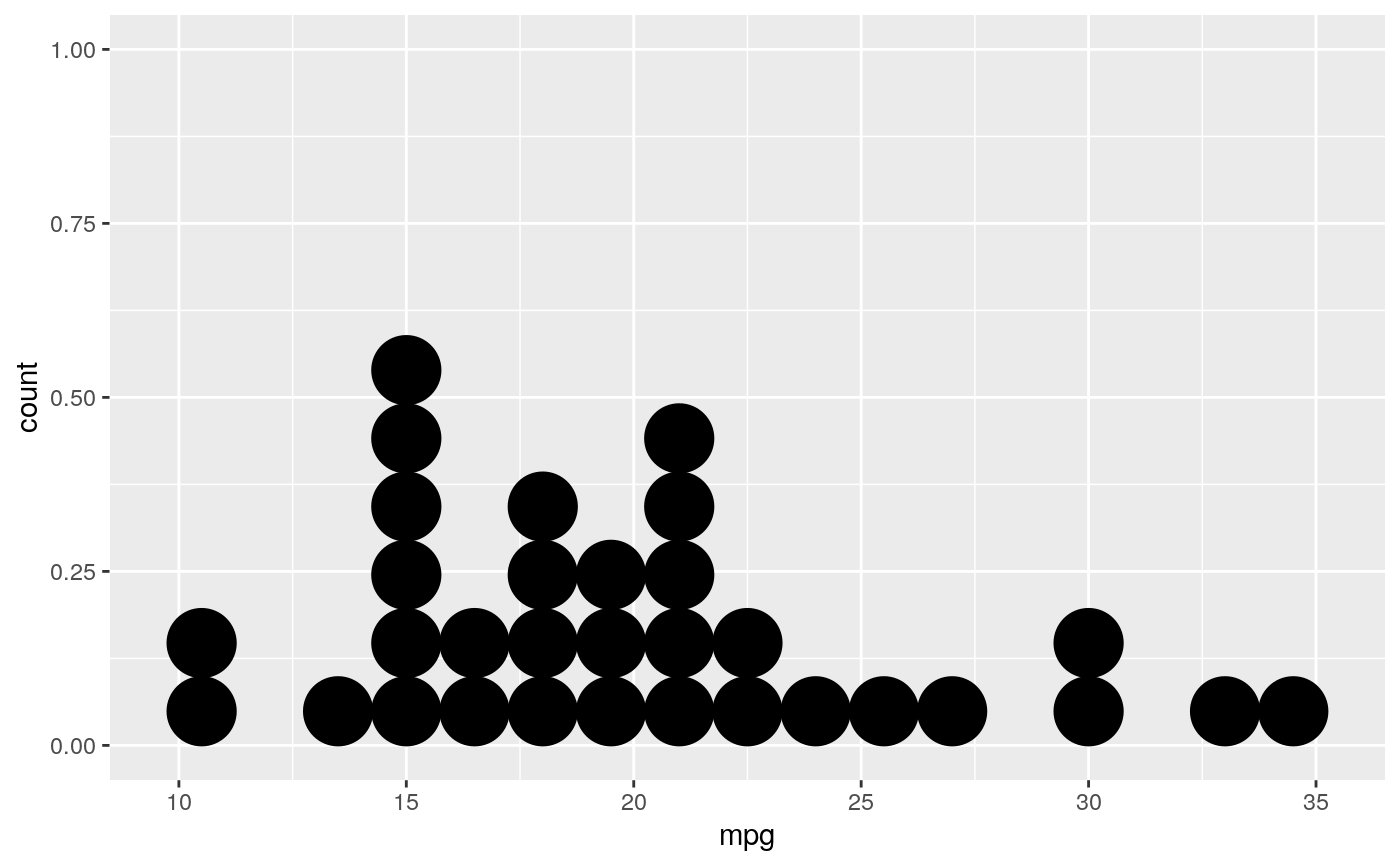
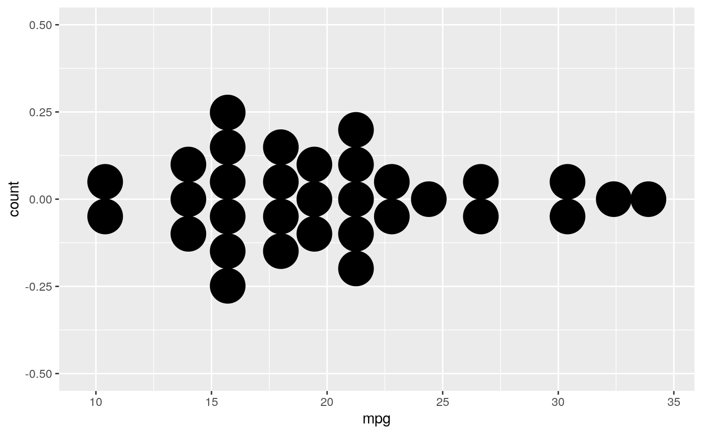
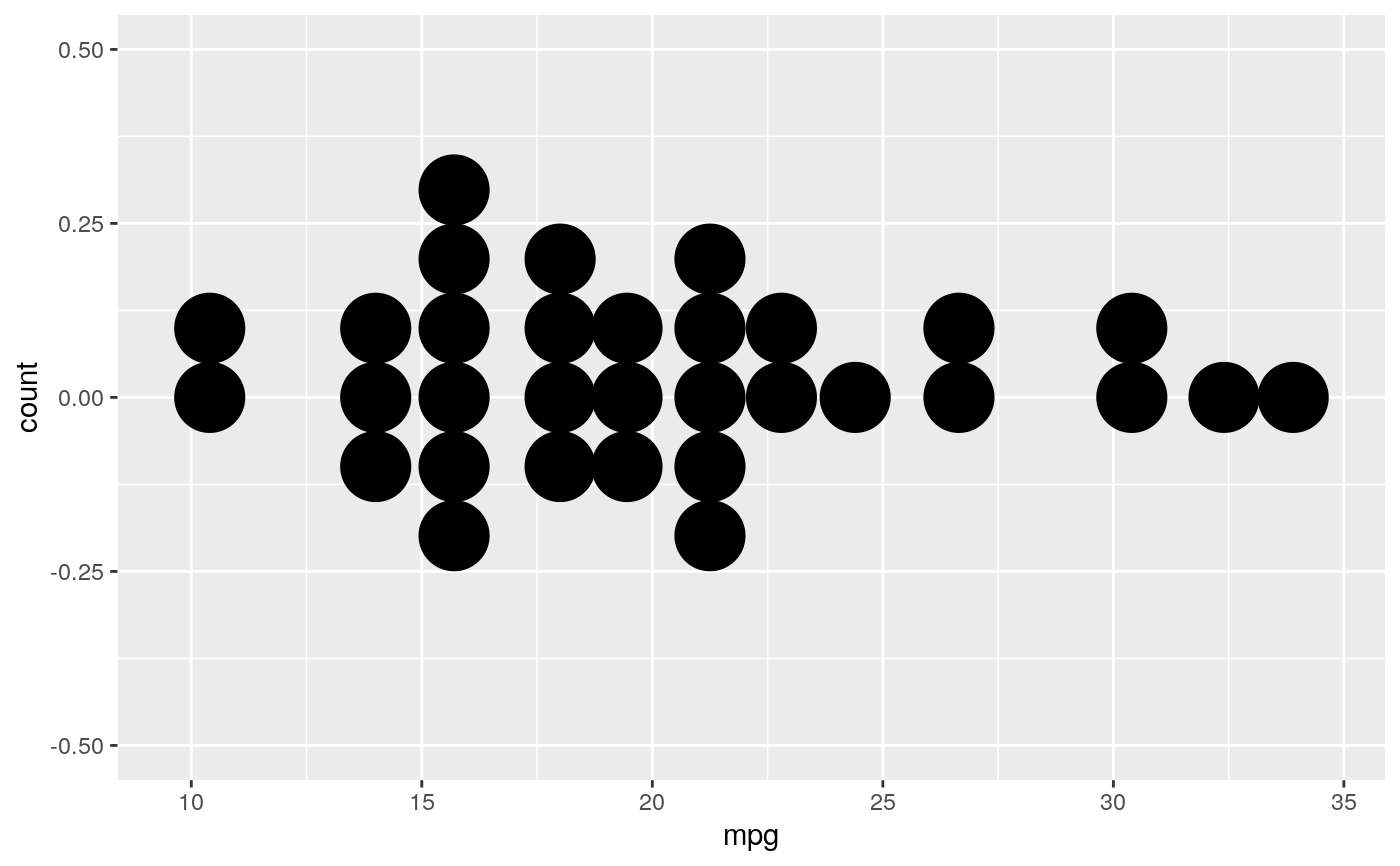
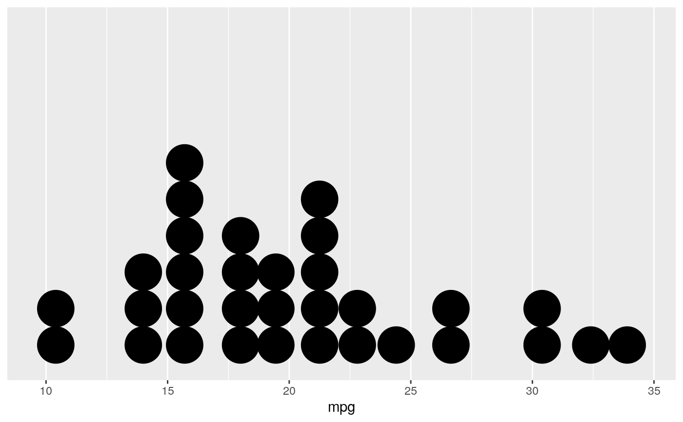
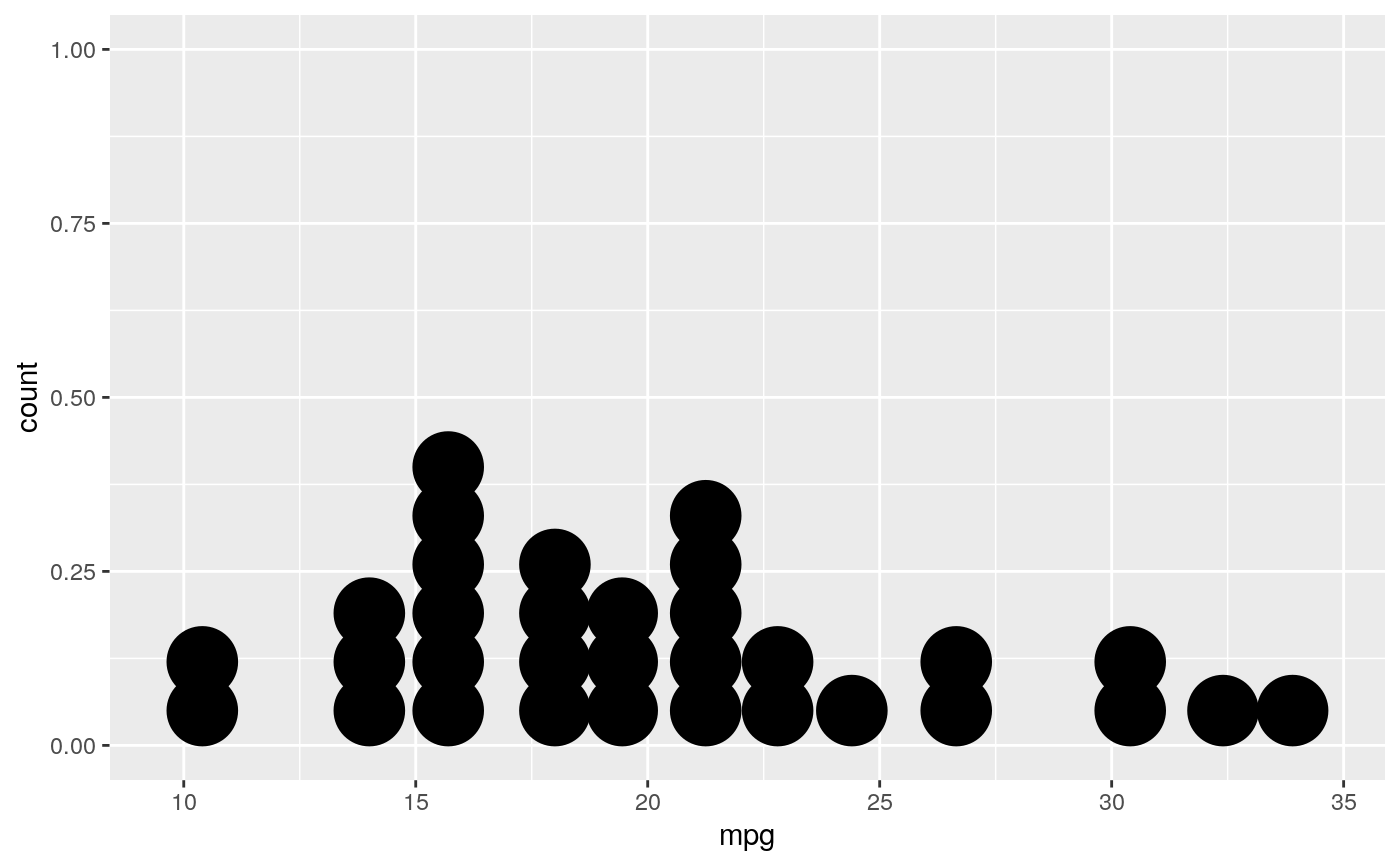
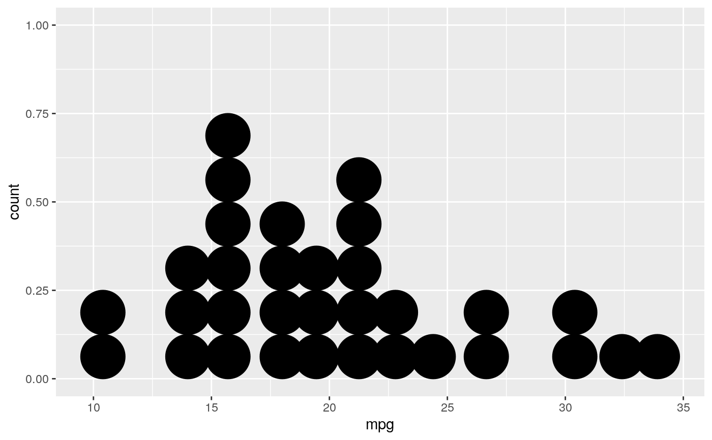
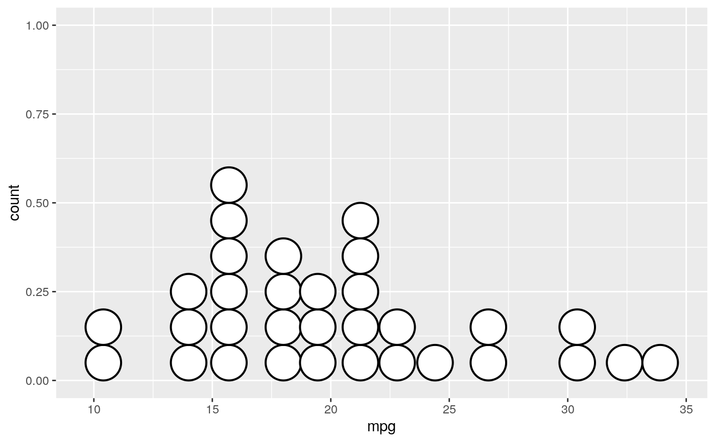
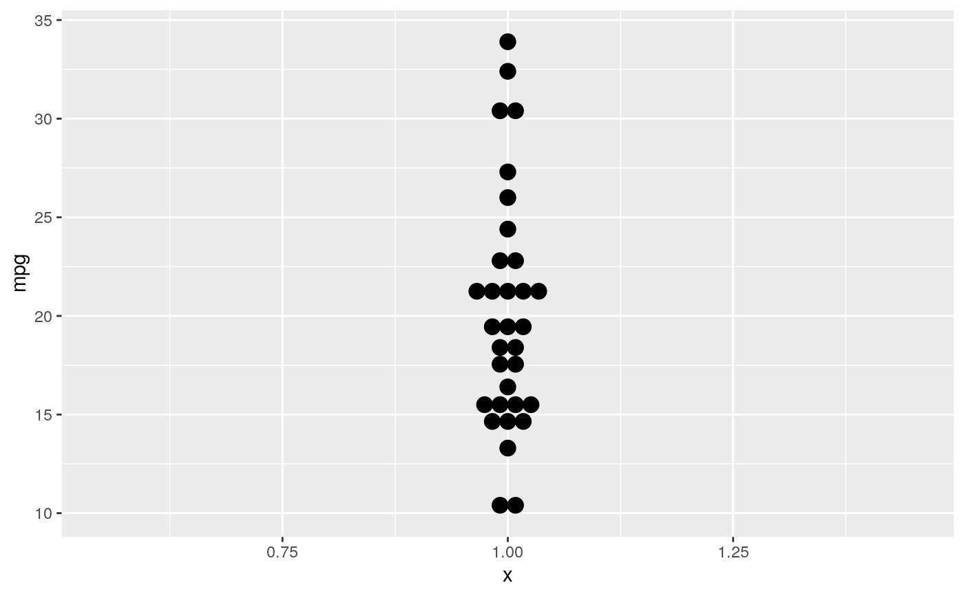
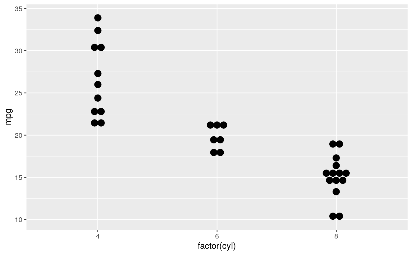
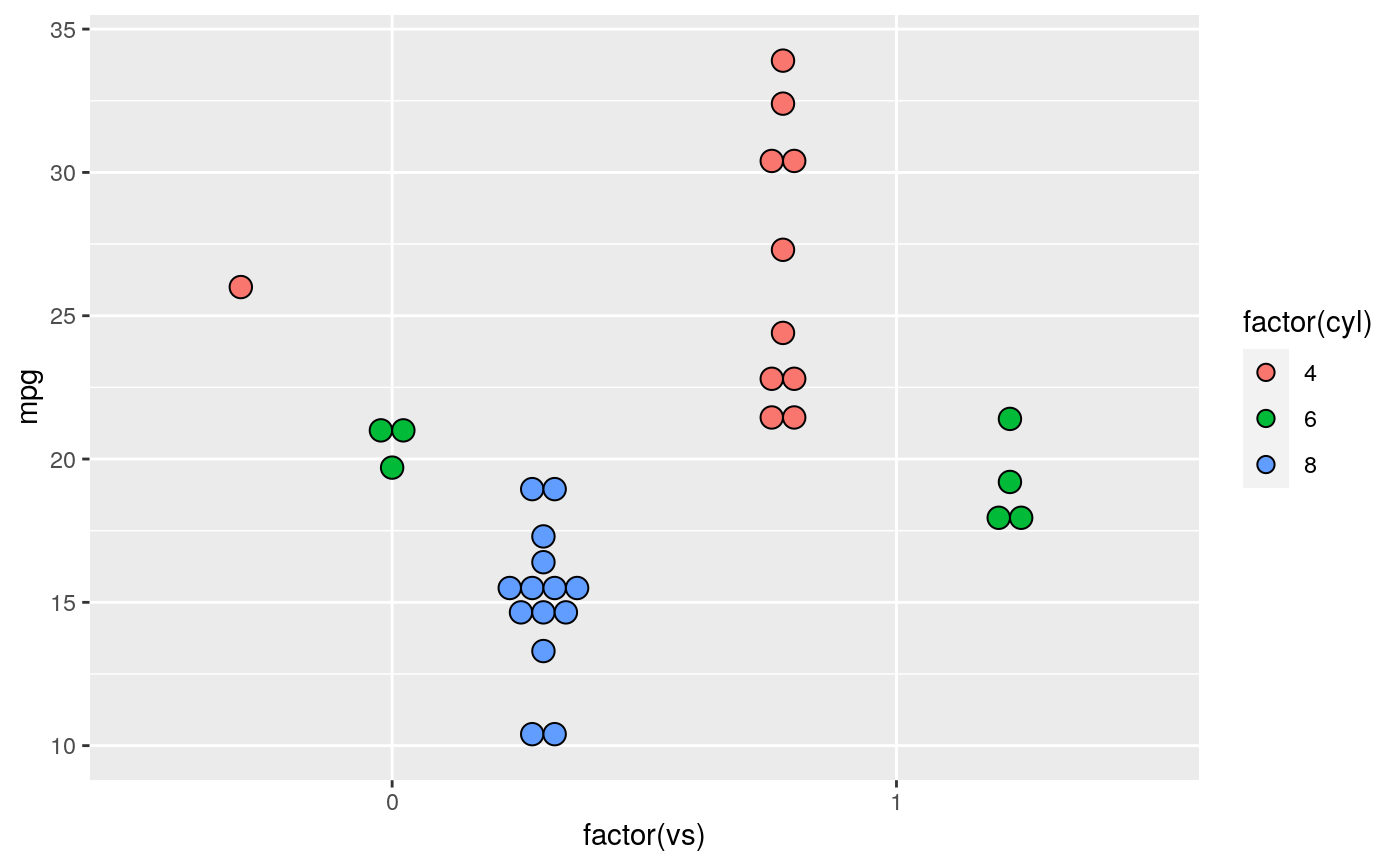
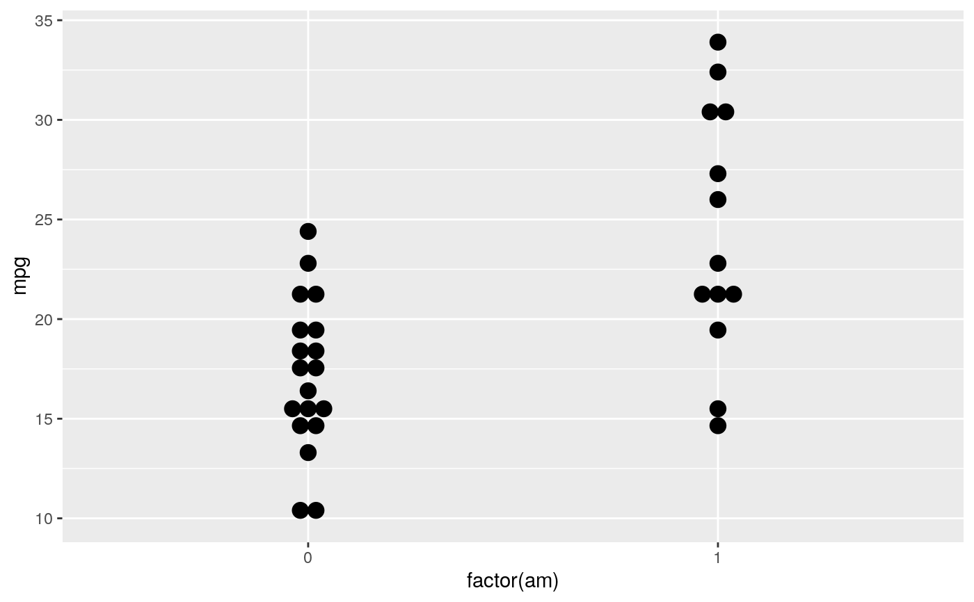
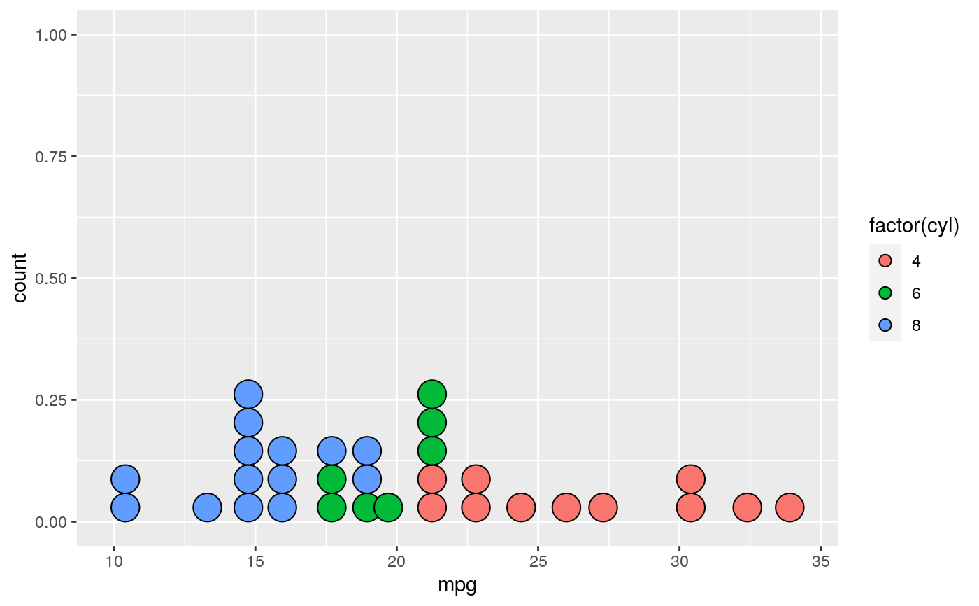
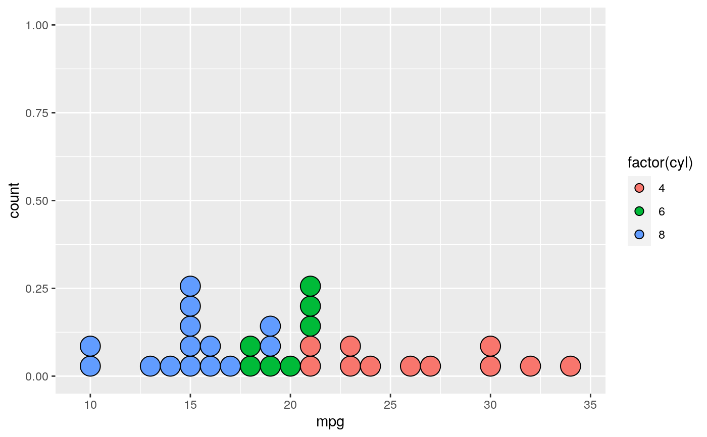
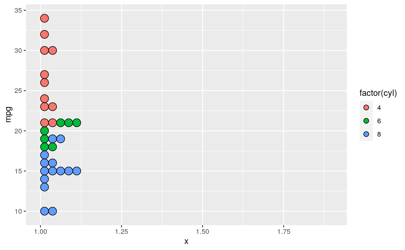
In a dot plot, the width of a dot corresponds to the bin width (or maximum width, depending on the binning algorithm), and dots are stacked, with each dot representing one observation.

geom_dotplot(
  mapping = NULL,
  data = NULL,
  position = "identity",
  ...,
  binwidth = NULL,
  binaxis = "x",
  method = "dotdensity",
  binpositions = "bygroup",
  stackdir = "up",
  stackratio = 1,
  dotsize = 1,
  stackgroups = FALSE,
  origin = NULL,
  right = TRUE,
  width = 0.9,
  drop = FALSE,
  na.rm = FALSE,
  show.legend = NA,
  inherit.aes = TRUE
)

Arguments

mapping	Set of aesthetic mappings created by `aes()` or `aes_()`. If specified and `inherit.aes = TRUE` (the default), it is combined with the default mapping at the top level of the plot. You must supply `mapping` if there is no plot mapping.
data	The data to be displayed in this layer. There are three options: If `NULL`, the default, the data is inherited from the plot data as specified in the call to `ggplot()`. A `data.frame`, or other object, will override the plot data. All objects will be fortified to produce a data frame. See `fortify()` for which variables will be created. A `function` will be called with a single argument, the plot data. The return value must be a `data.frame`, and will be used as the layer data. A `function` can be created from a `formula` (e.g. `~ head(.x, 10)`).
position	Position adjustment, either as a string, or the result of a call to a position adjustment function.
...	Other arguments passed on to `layer()`. These are often aesthetics, used to set an aesthetic to a fixed value, like `colour = "red"` or `size = 3`. They may also be parameters to the paired geom/stat.
binwidth	When `method` is "dotdensity", this specifies maximum bin width. When `method` is "histodot", this specifies bin width. Defaults to 1/30 of the range of the data
binaxis	The axis to bin along, "x" (default) or "y"
method	"dotdensity" (default) for dot-density binning, or "histodot" for fixed bin widths (like stat_bin)
binpositions	When `method` is "dotdensity", "bygroup" (default) determines positions of the bins for each group separately. "all" determines positions of the bins with all the data taken together; this is used for aligning dot stacks across multiple groups.
stackdir	which direction to stack the dots. "up" (default), "down", "center", "centerwhole" (centered, but with dots aligned)
stackratio	how close to stack the dots. Default is 1, where dots just touch. Use smaller values for closer, overlapping dots.
dotsize	The diameter of the dots relative to `binwidth`, default 1.
stackgroups	should dots be stacked across groups? This has the effect that `position = "stack"` should have, but can't (because this geom has some odd properties).
origin	When `method` is "histodot", origin of first bin
right	When `method` is "histodot", should intervals be closed on the right (a, b], or not [a, b)
width	When `binaxis` is "y", the spacing of the dot stacks for dodging.
drop	If TRUE, remove all bins with zero counts
na.rm	If `FALSE`, the default, missing values are removed with a warning. If `TRUE`, missing values are silently removed.
show.legend	logical. Should this layer be included in the legends? `NA`, the default, includes if any aesthetics are mapped. `FALSE` never includes, and `TRUE` always includes. It can also be a named logical vector to finely select the aesthetics to display.
inherit.aes	If `FALSE`, overrides the default aesthetics, rather than combining with them. This is most useful for helper functions that define both data and aesthetics and shouldn't inherit behaviour from the default plot specification, e.g. `borders()`.

Details

There are two basic approaches: dot-density and histodot. With dot-density binning, the bin positions are determined by the data and binwidth, which is the maximum width of each bin. See Wilkinson (1999) for details on the dot-density binning algorithm. With histodot binning, the bins have fixed positions and fixed widths, much like a histogram.

When binning along the x axis and stacking along the y axis, the numbers on y axis are not meaningful, due to technical limitations of ggplot2. You can hide the y axis, as in one of the examples, or manually scale it to match the number of dots.

Aesthetics

geom_dotplot() understands the following aesthetics (required aesthetics are in bold):

x
y
alpha
colour
fill
group
linetype
stroke

Learn more about setting these aesthetics in vignette("ggplot2-specs").

Computed variables

center of each bin, if binaxis is "x"

binwidth

max width of each bin if method is "dotdensity"; width of each bin if method is "histodot"

count

number of points in bin

ncount

count, scaled to maximum of 1

density

density of points in bin, scaled to integrate to 1, if method is "histodot"

ndensity

density, scaled to maximum of 1, if method is "histodot"

References

Wilkinson, L. (1999) Dot plots. The American Statistician, 53(3), 276-281.

Examples

ggplot(mtcars, aes(x = mpg)) + geom_dotplot()
#> `stat_bindot()` using `bins = 30`. Pick better value with `binwidth`.
ggplot(mtcars, aes(x = mpg)) + geom_dotplot(binwidth = 1.5)

# Use fixed-width bins
ggplot(mtcars, aes(x = mpg)) +
  geom_dotplot(method="histodot", binwidth = 1.5)

# Some other stacking methods
ggplot(mtcars, aes(x = mpg)) +
  geom_dotplot(binwidth = 1.5, stackdir = "center")
ggplot(mtcars, aes(x = mpg)) +
  geom_dotplot(binwidth = 1.5, stackdir = "centerwhole")

# y axis isn't really meaningful, so hide it
ggplot(mtcars, aes(x = mpg)) + geom_dotplot(binwidth = 1.5) +
  scale_y_continuous(NULL, breaks = NULL)

# Overlap dots vertically
ggplot(mtcars, aes(x = mpg)) + geom_dotplot(binwidth = 1.5, stackratio = .7)

# Expand dot diameter
ggplot(mtcars, aes(x = mpg)) + geom_dotplot(binwidth = 1.5, dotsize = 1.25)

# Change dot fill colour, stroke width
ggplot(mtcars, aes(x = mpg)) + geom_dotplot(binwidth = 1.5, fill = "white", stroke = 2)

# \donttest{
# Examples with stacking along y axis instead of x
ggplot(mtcars, aes(x = 1, y = mpg)) +
  geom_dotplot(binaxis = "y", stackdir = "center")
#> `stat_bindot()` using `bins = 30`. Pick better value with `binwidth`.

ggplot(mtcars, aes(x = factor(cyl), y = mpg)) +
  geom_dotplot(binaxis = "y", stackdir = "center")
#> `stat_bindot()` using `bins = 30`. Pick better value with `binwidth`.

ggplot(mtcars, aes(x = factor(cyl), y = mpg)) +
  geom_dotplot(binaxis = "y", stackdir = "centerwhole")
#> `stat_bindot()` using `bins = 30`. Pick better value with `binwidth`.

ggplot(mtcars, aes(x = factor(vs), fill = factor(cyl), y = mpg)) +
  geom_dotplot(binaxis = "y", stackdir = "center", position = "dodge")
#> `stat_bindot()` using `bins = 30`. Pick better value with `binwidth`.

# binpositions="all" ensures that the bins are aligned between groups
ggplot(mtcars, aes(x = factor(am), y = mpg)) +
  geom_dotplot(binaxis = "y", stackdir = "center", binpositions="all")
#> `stat_bindot()` using `bins = 30`. Pick better value with `binwidth`.

# Stacking multiple groups, with different fill
ggplot(mtcars, aes(x = mpg, fill = factor(cyl))) +
  geom_dotplot(stackgroups = TRUE, binwidth = 1, binpositions = "all")

ggplot(mtcars, aes(x = mpg, fill = factor(cyl))) +
  geom_dotplot(stackgroups = TRUE, binwidth = 1, method = "histodot")

ggplot(mtcars, aes(x = 1, y = mpg, fill = factor(cyl))) +
  geom_dotplot(binaxis = "y", stackgroups = TRUE, binwidth = 1, method = "histodot")
# }