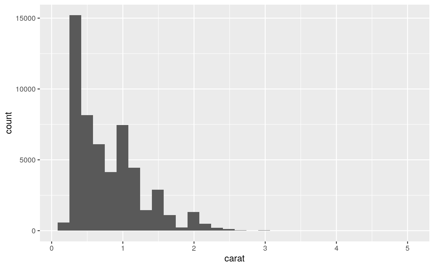
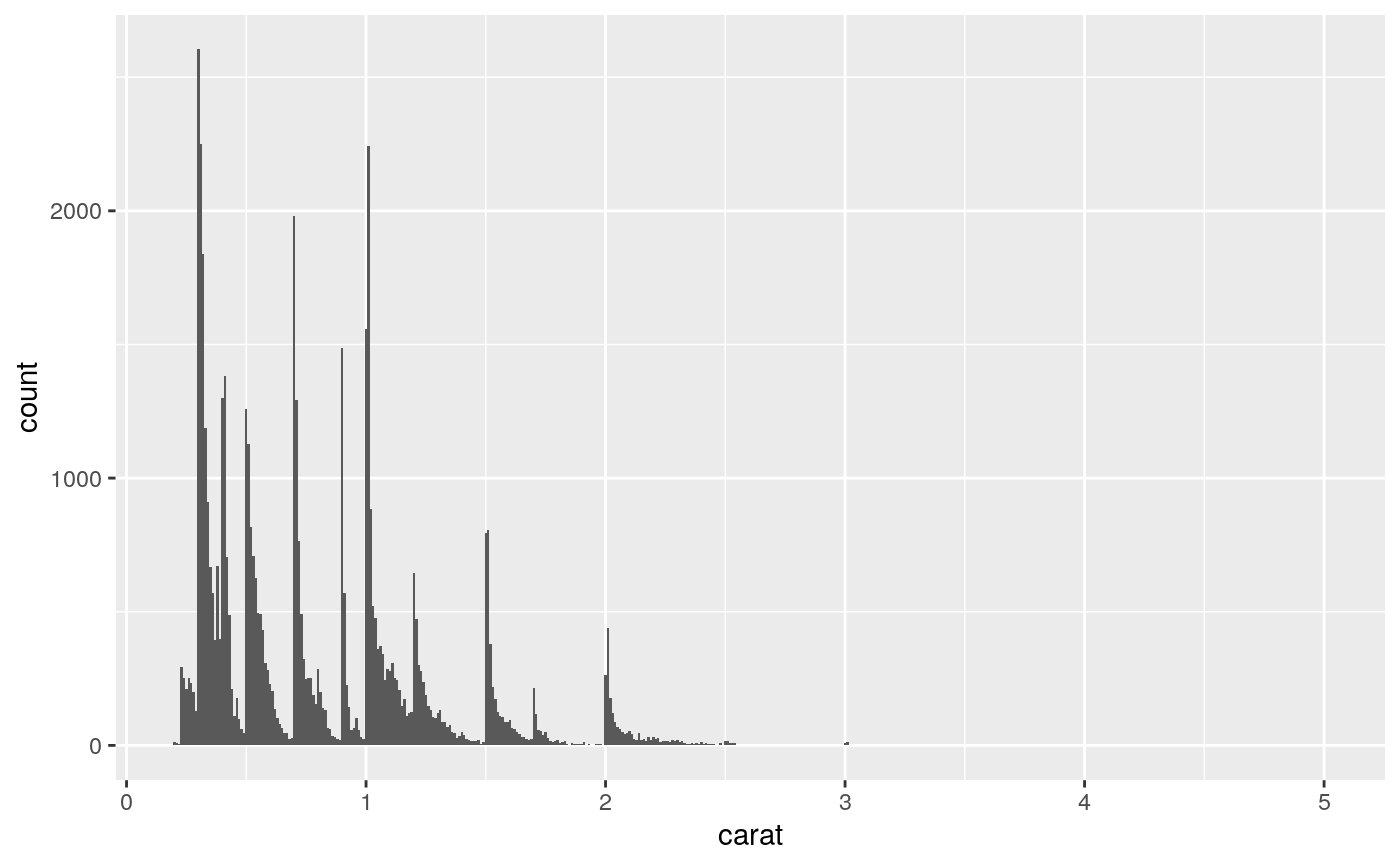
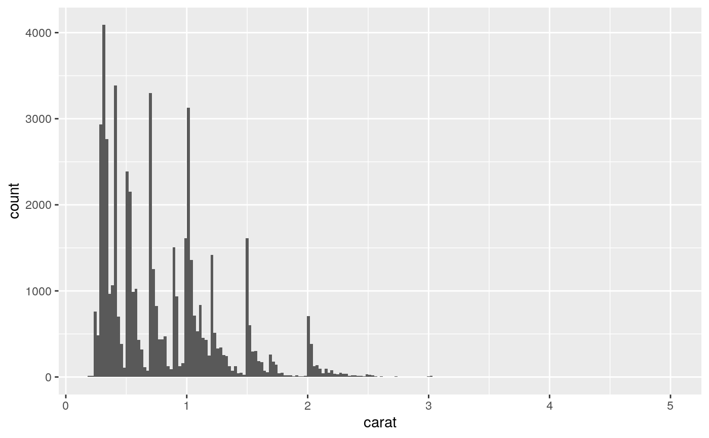
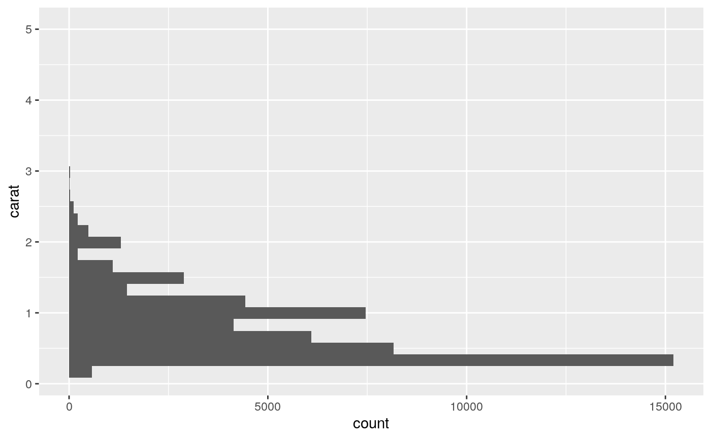
Histograms and frequency polygons

Visualise the distribution of a single continuous variable by dividing the x axis into bins and counting the number of observations in each bin. Histograms (geom_histogram()) display the counts with bars; frequency polygons (geom_freqpoly()) display the counts with lines. Frequency polygons are more suitable when you want to compare the distribution across the levels of a categorical variable.

geom_freqpoly(
  mapping = NULL,
  data = NULL,
  stat = "bin",
  position = "identity",
  ...,
  na.rm = FALSE,
  show.legend = NA,
  inherit.aes = TRUE
)

geom_histogram(
  mapping = NULL,
  data = NULL,
  stat = "bin",
  position = "stack",
  ...,
  binwidth = NULL,
  bins = NULL,
  na.rm = FALSE,
  orientation = NA,
  show.legend = NA,
  inherit.aes = TRUE
)

stat_bin(
  mapping = NULL,
  data = NULL,
  geom = "bar",
  position = "stack",
  ...,
  binwidth = NULL,
  bins = NULL,
  center = NULL,
  boundary = NULL,
  breaks = NULL,
  closed = c("right", "left"),
  pad = FALSE,
  na.rm = FALSE,
  orientation = NA,
  show.legend = NA,
  inherit.aes = TRUE
)

Arguments

mapping	Set of aesthetic mappings created by `aes()` or `aes_()`. If specified and `inherit.aes = TRUE` (the default), it is combined with the default mapping at the top level of the plot. You must supply `mapping` if there is no plot mapping.
data	The data to be displayed in this layer. There are three options: If `NULL`, the default, the data is inherited from the plot data as specified in the call to `ggplot()`. A `data.frame`, or other object, will override the plot data. All objects will be fortified to produce a data frame. See `fortify()` for which variables will be created. A `function` will be called with a single argument, the plot data. The return value must be a `data.frame`, and will be used as the layer data. A `function` can be created from a `formula` (e.g. `~ head(.x, 10)`).
position	Position adjustment, either as a string, or the result of a call to a position adjustment function.
...	Other arguments passed on to `layer()`. These are often aesthetics, used to set an aesthetic to a fixed value, like `colour = "red"` or `size = 3`. They may also be parameters to the paired geom/stat.
na.rm	If `FALSE`, the default, missing values are removed with a warning. If `TRUE`, missing values are silently removed.
show.legend	logical. Should this layer be included in the legends? `NA`, the default, includes if any aesthetics are mapped. `FALSE` never includes, and `TRUE` always includes. It can also be a named logical vector to finely select the aesthetics to display.
inherit.aes	If `FALSE`, overrides the default aesthetics, rather than combining with them. This is most useful for helper functions that define both data and aesthetics and shouldn't inherit behaviour from the default plot specification, e.g. `borders()`.
binwidth	The width of the bins. Can be specified as a numeric value or as a function that calculates width from unscaled x. Here, "unscaled x" refers to the original x values in the data, before application of any scale transformation. When specifying a function along with a grouping structure, the function will be called once per group. The default is to use the number of bins in `bins`, covering the range of the data. You should always override this value, exploring multiple widths to find the best to illustrate the stories in your data. The bin width of a date variable is the number of days in each time; the bin width of a time variable is the number of seconds.
bins	Number of bins. Overridden by `binwidth`. Defaults to 30.
orientation	The orientation of the layer. The default (`NA`) automatically determines the orientation from the aesthetic mapping. In the rare event that this fails it can be given explicitly by setting `orientation` to either `"x"` or `"y"`. See the Orientation section for more detail.
geom, stat	Use to override the default connection between `geom_histogram()`/`geom_freqpoly()` and `stat_bin()`.
center, boundary	bin position specifiers. Only one, `center` or `boundary`, may be specified for a single plot. `center` specifies the center of one of the bins. `boundary` specifies the boundary between two bins. Note that if either is above or below the range of the data, things will be shifted by the appropriate integer multiple of `width`. For example, to center on integers use `width = 1` and `center = 0`, even if `0` is outside the range of the data. Alternatively, this same alignment can be specified with `width = 1` and `boundary = 0.5`, even if `0.5` is outside the range of the data.
breaks	Alternatively, you can supply a numeric vector giving the bin boundaries. Overrides `binwidth`, `bins`, `center`, and `boundary`.
closed	One of `"right"` or `"left"` indicating whether right or left edges of bins are included in the bin.
pad	If `TRUE`, adds empty bins at either end of x. This ensures frequency polygons touch 0. Defaults to `FALSE`.

Details

stat_bin() is suitable only for continuous x data. If your x data is discrete, you probably want to use stat_count().

By default, the underlying computation (stat_bin()) uses 30 bins; this is not a good default, but the idea is to get you experimenting with different number of bins. You can also experiment modifying the binwidth with center or boundary arguments. binwidth overrides bins so you should do one change at a time. You may need to look at a few options to uncover the full story behind your data.

Orientation

This geom treats each axis differently and, thus, can thus have two orientations. Often the orientation is easy to deduce from a combination of the given mappings and the types of positional scales in use. Thus, ggplot2 will by default try to guess which orientation the layer should have. Under rare circumstances, the orientation is ambiguous and guessing may fail. In that case the orientation can be specified directly using the orientation parameter, which can be either "x" or "y". The value gives the axis that the geom should run along, "x" being the default orientation you would expect for the geom.

Aesthetics

geom_histogram() uses the same aesthetics as geom_bar(); geom_freqpoly() uses the same aesthetics as geom_line().

Computed variables

count

number of points in bin

density

density of points in bin, scaled to integrate to 1

ncount

count, scaled to maximum of 1

ndensity

density, scaled to maximum of 1

Examples

ggplot(diamonds, aes(carat)) +
  geom_histogram()
#> `stat_bin()` using `bins = 30`. Pick better value with `binwidth`.
ggplot(diamonds, aes(carat)) +
  geom_histogram(binwidth = 0.01)
ggplot(diamonds, aes(carat)) +
  geom_histogram(bins = 200)
# Map values to y to flip the orientation
ggplot(diamonds, aes(y = carat)) +
  geom_histogram()
#> `stat_bin()` using `bins = 30`. Pick better value with `binwidth`.

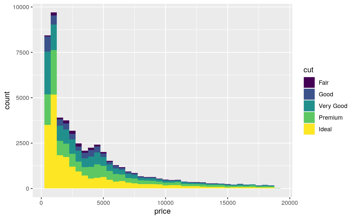
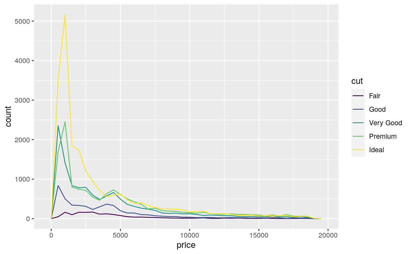
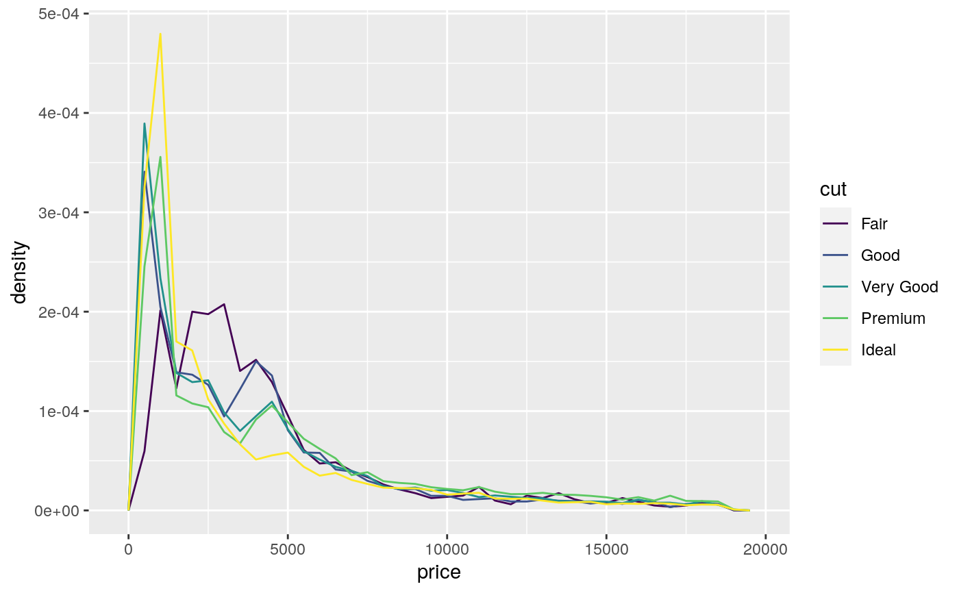
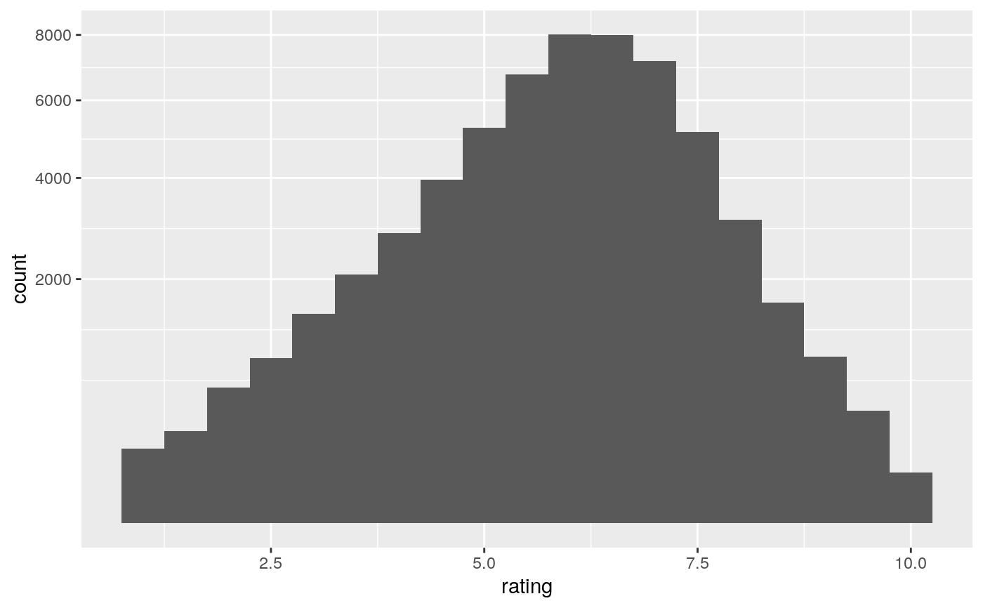
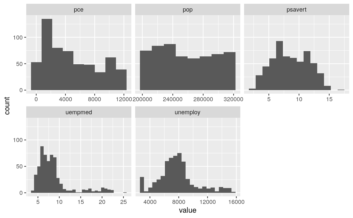
# Rather than stacking histograms, it's easier to compare frequency
# polygons
ggplot(diamonds, aes(price, fill = cut)) +
  geom_histogram(binwidth = 500)
ggplot(diamonds, aes(price, colour = cut)) +
  geom_freqpoly(binwidth = 500)

# To make it easier to compare distributions with very different counts,
# put density on the y axis instead of the default count
ggplot(diamonds, aes(price, after_stat(density), colour = cut)) +
  geom_freqpoly(binwidth = 500)

if (require("ggplot2movies")) {
# Often we don't want the height of the bar to represent the
# count of observations, but the sum of some other variable.
# For example, the following plot shows the number of movies
# in each rating.
m <- ggplot(movies, aes(rating))
m + geom_histogram(binwidth = 0.1)

# If, however, we want to see the number of votes cast in each
# category, we need to weight by the votes variable
m + geom_histogram(aes(weight = votes), binwidth = 0.1) + ylab("votes")

# For transformed scales, binwidth applies to the transformed data.
# The bins have constant width on the transformed scale.
m + geom_histogram() + scale_x_log10()
m + geom_histogram(binwidth = 0.05) + scale_x_log10()

# For transformed coordinate systems, the binwidth applies to the
# raw data. The bins have constant width on the original scale.

# Using log scales does not work here, because the first
# bar is anchored at zero, and so when transformed becomes negative
# infinity. This is not a problem when transforming the scales, because
# no observations have 0 ratings.
m + geom_histogram(boundary = 0) + coord_trans(x = "log10")
# Use boundary = 0, to make sure we don't take sqrt of negative values
m + geom_histogram(boundary = 0) + coord_trans(x = "sqrt")

# You can also transform the y axis.  Remember that the base of the bars
# has value 0, so log transformations are not appropriate
m <- ggplot(movies, aes(x = rating))
m + geom_histogram(binwidth = 0.5) + scale_y_sqrt()
}

# You can specify a function for calculating binwidth, which is
# particularly useful when faceting along variables with
# different ranges because the function will be called once per facet
ggplot(economics_long, aes(value)) +
  facet_wrap(~variable, scales = 'free_x') +
  geom_histogram(binwidth = function(x) 2 * IQR(x) / (length(x)^(1/3)))