Polygons

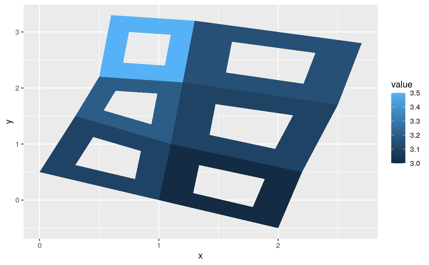
Polygons are very similar to paths (as drawn by geom_path()) except that the start and end points are connected and the inside is coloured by fill. The group aesthetic determines which cases are connected together into a polygon. From R 3.6 and onwards it is possible to draw polygons with holes by providing a subgroup aesthetic that differentiates the outer ring points from those describing holes in the polygon.

geom_polygon(
  mapping = NULL,
  data = NULL,
  stat = "identity",
  position = "identity",
  rule = "evenodd",
  ...,
  na.rm = FALSE,
  show.legend = NA,
  inherit.aes = TRUE
)

Arguments

mapping	Set of aesthetic mappings created by `aes()` or `aes_()`. If specified and `inherit.aes = TRUE` (the default), it is combined with the default mapping at the top level of the plot. You must supply `mapping` if there is no plot mapping.
data	The data to be displayed in this layer. There are three options: If `NULL`, the default, the data is inherited from the plot data as specified in the call to `ggplot()`. A `data.frame`, or other object, will override the plot data. All objects will be fortified to produce a data frame. See `fortify()` for which variables will be created. A `function` will be called with a single argument, the plot data. The return value must be a `data.frame`, and will be used as the layer data. A `function` can be created from a `formula` (e.g. `~ head(.x, 10)`).
stat	The statistical transformation to use on the data for this layer, as a string.
position	Position adjustment, either as a string, or the result of a call to a position adjustment function.
rule	Either `"evenodd"` or `"winding"`. If polygons with holes are being drawn (using the `subgroup` aesthetic) this argument defines how the hole coordinates are interpreted. See the examples in `grid::pathGrob()` for an explanation.
...	Other arguments passed on to `layer()`. These are often aesthetics, used to set an aesthetic to a fixed value, like `colour = "red"` or `size = 3`. They may also be parameters to the paired geom/stat.
na.rm	If `FALSE`, the default, missing values are removed with a warning. If `TRUE`, missing values are silently removed.
show.legend	logical. Should this layer be included in the legends? `NA`, the default, includes if any aesthetics are mapped. `FALSE` never includes, and `TRUE` always includes. It can also be a named logical vector to finely select the aesthetics to display.
inherit.aes	If `FALSE`, overrides the default aesthetics, rather than combining with them. This is most useful for helper functions that define both data and aesthetics and shouldn't inherit behaviour from the default plot specification, e.g. `borders()`.

Aesthetics

geom_polygon() understands the following aesthetics (required aesthetics are in bold):

x
y
alpha
colour
fill
group
linetype
size
subgroup

Learn more about setting these aesthetics in vignette("ggplot2-specs").

Examples

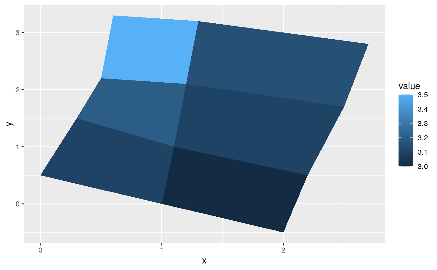
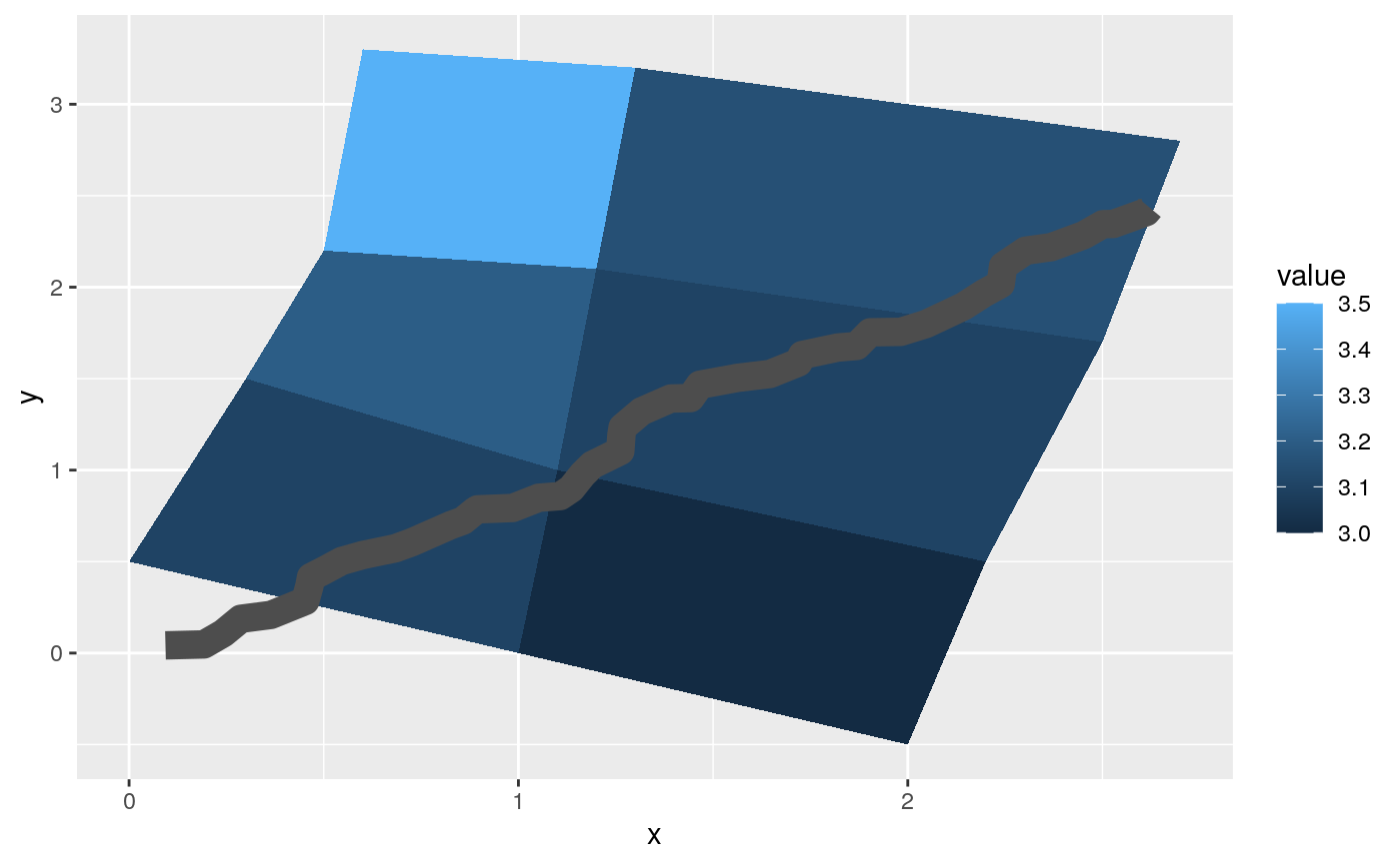
# When using geom_polygon, you will typically need two data frames:
# one contains the coordinates of each polygon (positions),  and the
# other the values associated with each polygon (values).  An id
# variable links the two together

ids <- factor(c("1.1", "2.1", "1.2", "2.2", "1.3", "2.3"))

values <- data.frame(
  id = ids,
  value = c(3, 3.1, 3.1, 3.2, 3.15, 3.5)
)

positions <- data.frame(
  id = rep(ids, each = 4),
  x = c(2, 1, 1.1, 2.2, 1, 0, 0.3, 1.1, 2.2, 1.1, 1.2, 2.5, 1.1, 0.3,
  0.5, 1.2, 2.5, 1.2, 1.3, 2.7, 1.2, 0.5, 0.6, 1.3),
  y = c(-0.5, 0, 1, 0.5, 0, 0.5, 1.5, 1, 0.5, 1, 2.1, 1.7, 1, 1.5,
  2.2, 2.1, 1.7, 2.1, 3.2, 2.8, 2.1, 2.2, 3.3, 3.2)
)

# Currently we need to manually merge the two together
datapoly <- merge(values, positions, by = c("id"))

p <- ggplot(datapoly, aes(x = x, y = y)) +
  geom_polygon(aes(fill = value, group = id))
p

# Which seems like a lot of work, but then it's easy to add on
# other features in this coordinate system, e.g.:

stream <- data.frame(
  x = cumsum(runif(50, max = 0.1)),
  y = cumsum(runif(50,max = 0.1))
)

p + geom_line(data = stream, colour = "grey30", size = 5)

# And if the positions are in longitude and latitude, you can use
# coord_map to produce different map projections.

if (packageVersion("grid") >= "3.6") {
  # As of R version 3.6 geom_polygon() supports polygons with holes
  # Use the subgroup aesthetic to differentiate holes from the main polygon

  holes <- do.call(rbind, lapply(split(datapoly, datapoly$id), function(df) {
    df$x <- df$x + 0.5 * (mean(df$x) - df$x)
    df$y <- df$y + 0.5 * (mean(df$y) - df$y)
    df
  }))
  datapoly$subid <- 1L
  holes$subid <- 2L
  datapoly <- rbind(datapoly, holes)

  p <- ggplot(datapoly, aes(x = x, y = y)) +
    geom_polygon(aes(fill = value, group = id, subgroup = subid))
  p
}

Arguments

Aesthetics

See also

Examples