A quantile-quantile plot

geom_qq and stat_qq produce quantile-quantile plots. geom_qq_line and stat_qq_line compute the slope and intercept of the line connecting the points at specified quartiles of the theoretical and sample distributions.

geom_qq_line(
  mapping = NULL,
  data = NULL,
  geom = "path",
  position = "identity",
  ...,
  distribution = stats::qnorm,
  dparams = list(),
  line.p = c(0.25, 0.75),
  fullrange = FALSE,
  na.rm = FALSE,
  show.legend = NA,
  inherit.aes = TRUE
)

stat_qq_line(
  mapping = NULL,
  data = NULL,
  geom = "path",
  position = "identity",
  ...,
  distribution = stats::qnorm,
  dparams = list(),
  line.p = c(0.25, 0.75),
  fullrange = FALSE,
  na.rm = FALSE,
  show.legend = NA,
  inherit.aes = TRUE
)

geom_qq(
  mapping = NULL,
  data = NULL,
  geom = "point",
  position = "identity",
  ...,
  distribution = stats::qnorm,
  dparams = list(),
  na.rm = FALSE,
  show.legend = NA,
  inherit.aes = TRUE
)

stat_qq(
  mapping = NULL,
  data = NULL,
  geom = "point",
  position = "identity",
  ...,
  distribution = stats::qnorm,
  dparams = list(),
  na.rm = FALSE,
  show.legend = NA,
  inherit.aes = TRUE
)

Arguments

mapping	Set of aesthetic mappings created by aes() or aes_(). If specified and inherit.aes = TRUE (the default), it is combined with the default mapping at the top level of the plot. You must supply mapping if there is no plot mapping.
data	The data to be displayed in this layer. There are three options: If NULL, the default, the data is inherited from the plot data as specified in the call to ggplot(). A data.frame, or other object, will override the plot data. All objects will be fortified to produce a data frame. See fortify() for which variables will be created. A function will be called with a single argument, the plot data. The return value must be a data.frame, and will be used as the layer data. A function can be created from a formula (e.g. ~ head(.x, 10)).
geom	The geometric object to use display the data
position	Position adjustment, either as a string, or the result of a call to a position adjustment function.
...	Other arguments passed on to layer(). These are often aesthetics, used to set an aesthetic to a fixed value, like colour = "red" or size = 3. They may also be parameters to the paired geom/stat.
distribution	Distribution function to use, if x not specified
dparams	Additional parameters passed on to distribution function.
line.p	Vector of quantiles to use when fitting the Q-Q line, defaults defaults to c(.25, .75).
fullrange	Should the q-q line span the full range of the plot, or just the data
na.rm	If FALSE, the default, missing values are removed with a warning. If TRUE, missing values are silently removed.
show.legend	logical. Should this layer be included in the legends? NA, the default, includes if any aesthetics are mapped. FALSE never includes, and TRUE always includes. It can also be a named logical vector to finely select the aesthetics to display.
inherit.aes	If FALSE, overrides the default aesthetics, rather than combining with them. This is most useful for helper functions that define both data and aesthetics and shouldn't inherit behaviour from the default plot specification, e.g. borders().

Aesthetics

stat_qq() understands the following aesthetics (required aesthetics are in bold):

• sample

• group

• x

• y

Learn more about setting these aesthetics in vignette("ggplot2-specs").

stat_qq_line() understands the following aesthetics (required aesthetics are in bold):

• sample

• group

• x

• y

Learn more about setting these aesthetics in vignette("ggplot2-specs").

Computed variables

Variables computed by stat_qq:

sample

sample quantiles

theoretical

theoretical quantiles

Variables computed by stat_qq_line:

x

x-coordinates of the endpoints of the line segment connecting the points at the chosen quantiles of the theoretical and the sample distributions

y

y-coordinates of the endpoints

Examples

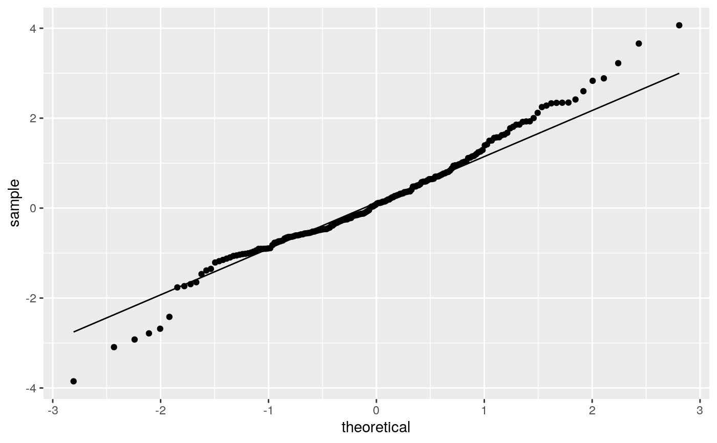
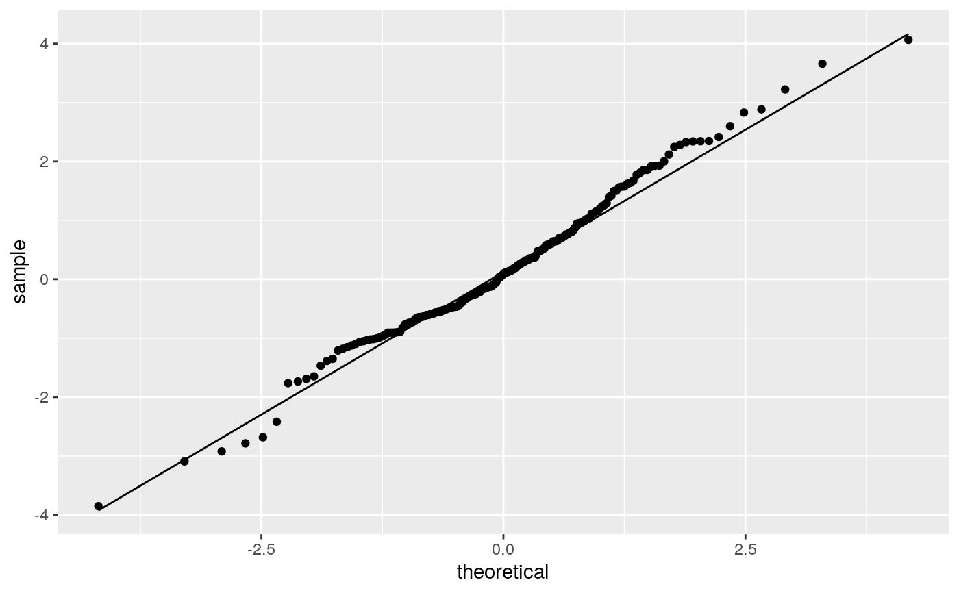
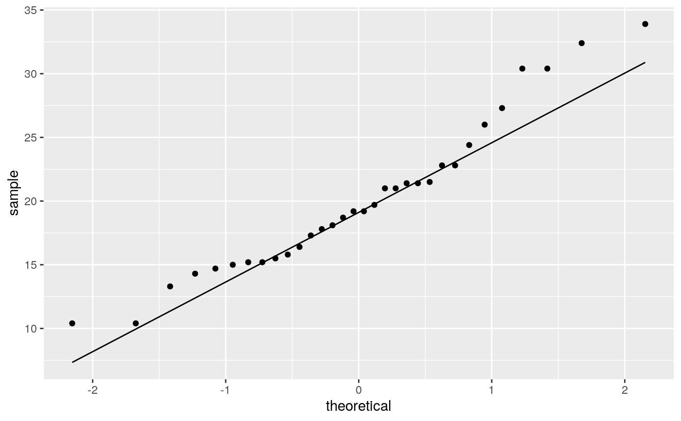
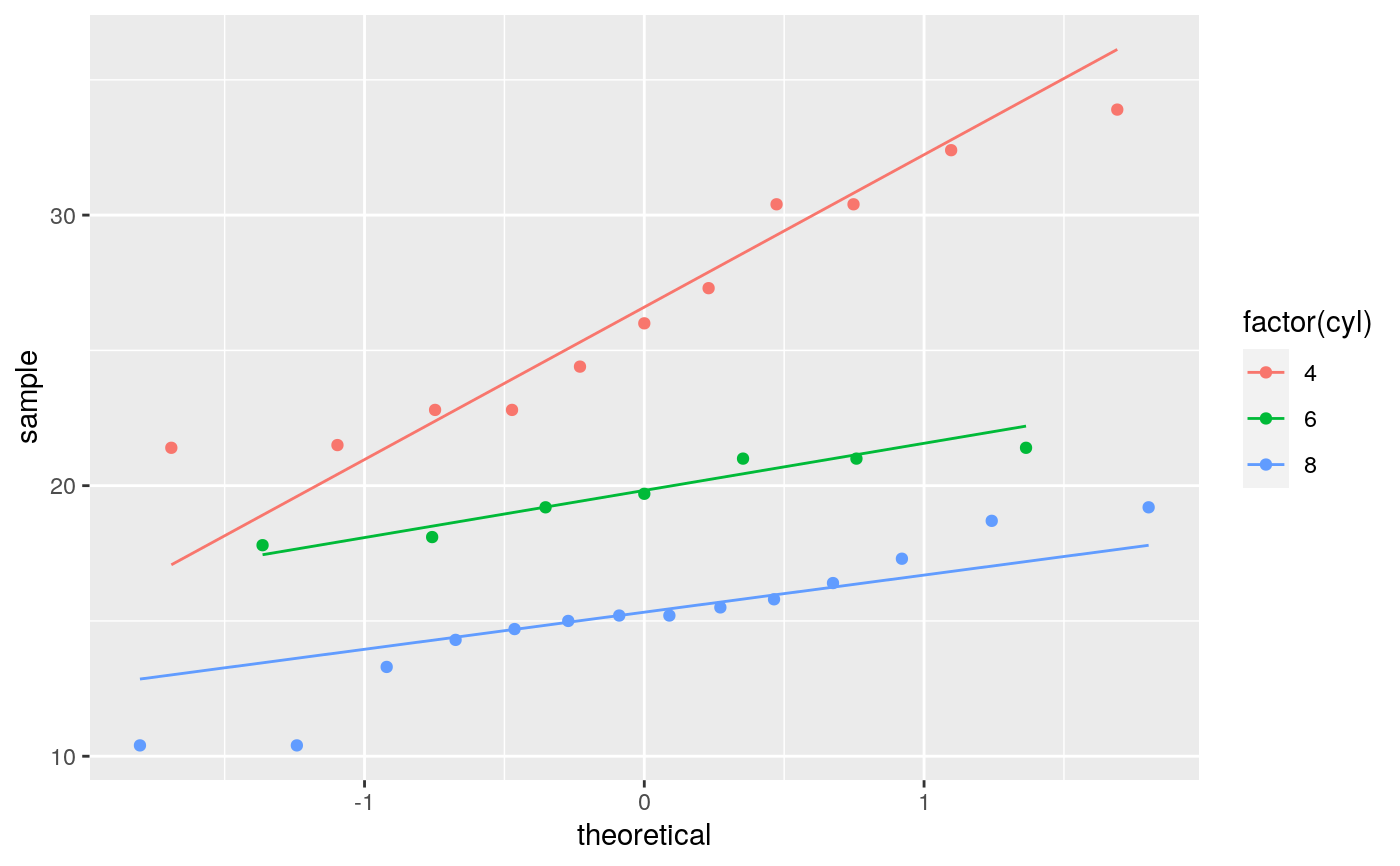
# \donttest{
df <- data.frame(y = rt(200, df = 5))
p <- ggplot(df, aes(sample = y))
p + stat_qq() + stat_qq_line()

# Use fitdistr from MASS to estimate distribution params
params <- as.list(MASS::fitdistr(df$y, "t")$estimate)
ggplot(df, aes(sample = y)) +
  stat_qq(distribution = qt, dparams = params["df"]) +
  stat_qq_line(distribution = qt, dparams = params["df"])

# Using to explore the distribution of a variable
ggplot(mtcars, aes(sample = mpg)) +
  stat_qq() +
  stat_qq_line()
ggplot(mtcars, aes(sample = mpg, colour = factor(cyl))) +
  stat_qq() +
  stat_qq_line()
# }