Smoothed conditional means

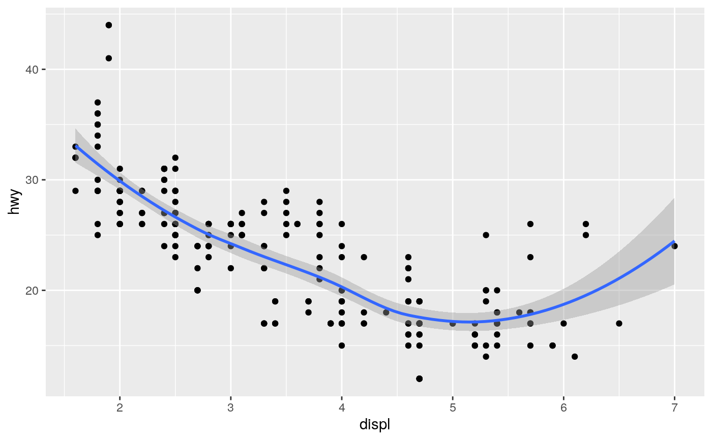
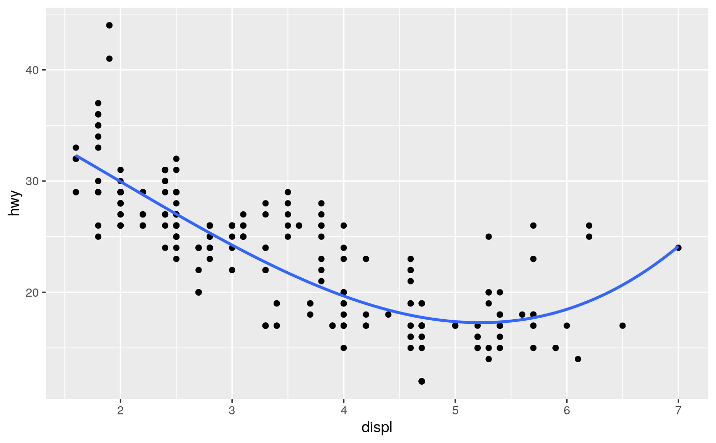
Aids the eye in seeing patterns in the presence of overplotting. geom_smooth() and stat_smooth() are effectively aliases: they both use the same arguments. Use stat_smooth() if you want to display the results with a non-standard geom.

geom_smooth(
  mapping = NULL,
  data = NULL,
  stat = "smooth",
  position = "identity",
  ...,
  method = NULL,
  formula = NULL,
  se = TRUE,
  na.rm = FALSE,
  orientation = NA,
  show.legend = NA,
  inherit.aes = TRUE
)

stat_smooth(
  mapping = NULL,
  data = NULL,
  geom = "smooth",
  position = "identity",
  ...,
  method = NULL,
  formula = NULL,
  se = TRUE,
  n = 80,
  span = 0.75,
  fullrange = FALSE,
  level = 0.95,
  method.args = list(),
  na.rm = FALSE,
  orientation = NA,
  show.legend = NA,
  inherit.aes = TRUE
)

Arguments

mapping	Set of aesthetic mappings created by `aes()` or `aes_()`. If specified and `inherit.aes = TRUE` (the default), it is combined with the default mapping at the top level of the plot. You must supply `mapping` if there is no plot mapping.
data	The data to be displayed in this layer. There are three options: If `NULL`, the default, the data is inherited from the plot data as specified in the call to `ggplot()`. A `data.frame`, or other object, will override the plot data. All objects will be fortified to produce a data frame. See `fortify()` for which variables will be created. A `function` will be called with a single argument, the plot data. The return value must be a `data.frame`, and will be used as the layer data. A `function` can be created from a `formula` (e.g. `~ head(.x, 10)`).
position	Position adjustment, either as a string, or the result of a call to a position adjustment function.
...	Other arguments passed on to `layer()`. These are often aesthetics, used to set an aesthetic to a fixed value, like `colour = "red"` or `size = 3`. They may also be parameters to the paired geom/stat.
method	Smoothing method (function) to use, accepts either `NULL` or a character vector, e.g. `"lm"`, `"glm"`, `"gam"`, `"loess"` or a function, e.g. `MASS::rlm` or `mgcv::gam`, `stats::lm`, or `stats::loess`. `"auto"` is also accepted for backwards compatibility. It is equivalent to `NULL`. For `method = NULL` the smoothing method is chosen based on the size of the largest group (across all panels). `stats::loess()` is used for less than 1,000 observations; otherwise `mgcv::gam()` is used with `formula = y ~ s(x, bs = "cs")` with `method = "REML"`. Somewhat anecdotally, `loess` gives a better appearance, but is \(O(N^{2})\) in memory, so does not work for larger datasets. If you have fewer than 1,000 observations but want to use the same `gam()` model that `method = NULL` would use, then set `method = "gam", formula = y ~ s(x, bs = "cs")`.
formula	Formula to use in smoothing function, eg. `y ~ x`, `y ~ poly(x, 2)`, `y ~ log(x)`. `NULL` by default, in which case `method = NULL` implies `formula = y ~ x` when there are fewer than 1,000 observations and `formula = y ~ s(x, bs = "cs")` otherwise.
se	Display confidence interval around smooth? (`TRUE` by default, see `level` to control.)
na.rm	If `FALSE`, the default, missing values are removed with a warning. If `TRUE`, missing values are silently removed.
orientation	The orientation of the layer. The default (`NA`) automatically determines the orientation from the aesthetic mapping. In the rare event that this fails it can be given explicitly by setting `orientation` to either `"x"` or `"y"`. See the Orientation section for more detail.
show.legend	logical. Should this layer be included in the legends? `NA`, the default, includes if any aesthetics are mapped. `FALSE` never includes, and `TRUE` always includes. It can also be a named logical vector to finely select the aesthetics to display.
inherit.aes	If `FALSE`, overrides the default aesthetics, rather than combining with them. This is most useful for helper functions that define both data and aesthetics and shouldn't inherit behaviour from the default plot specification, e.g. `borders()`.
geom, stat	Use to override the default connection between `geom_smooth()` and `stat_smooth()`.
n	Number of points at which to evaluate smoother.
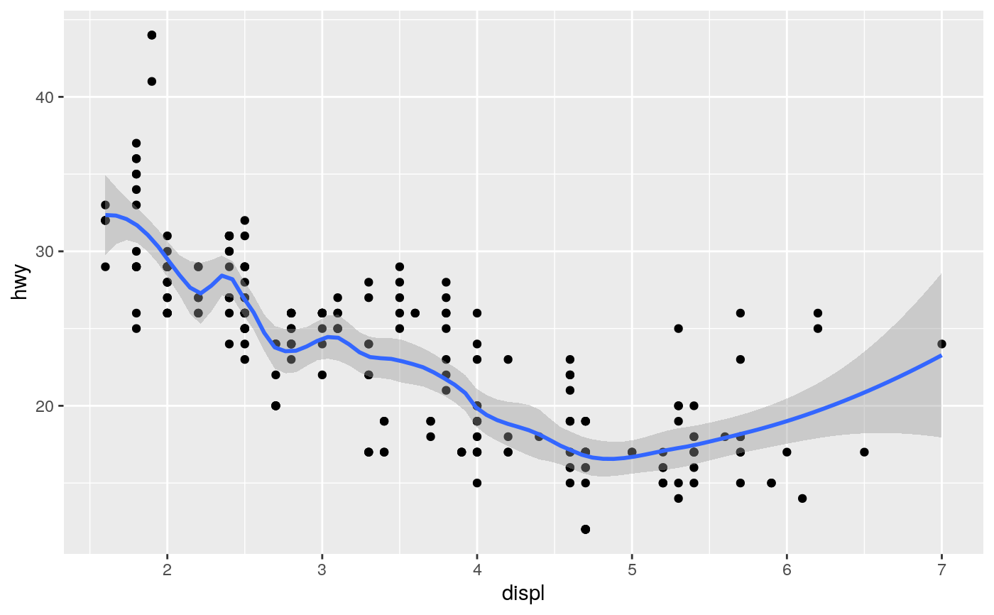
span	Controls the amount of smoothing for the default loess smoother. Smaller numbers produce wigglier lines, larger numbers produce smoother lines.
fullrange	Should the fit span the full range of the plot, or just the data?
level	Level of confidence interval to use (0.95 by default).
method.args	List of additional arguments passed on to the modelling function defined by `method`.

Details

Calculation is performed by the (currently undocumented) predictdf() generic and its methods. For most methods the standard error bounds are computed using the predict() method -- the exceptions are loess(), which uses a t-based approximation, and glm(), where the normal confidence interval is constructed on the link scale and then back-transformed to the response scale.

Orientation

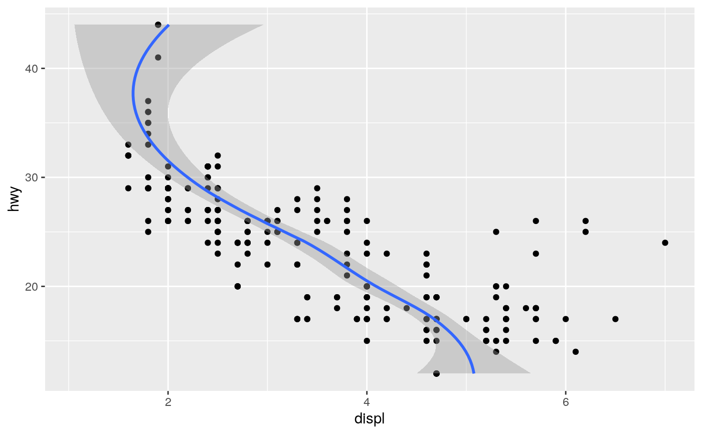
This geom treats each axis differently and, thus, can thus have two orientations. Often the orientation is easy to deduce from a combination of the given mappings and the types of positional scales in use. Thus, ggplot2 will by default try to guess which orientation the layer should have. Under rare circumstances, the orientation is ambiguous and guessing may fail. In that case the orientation can be specified directly using the orientation parameter, which can be either "x" or "y". The value gives the axis that the geom should run along, "x" being the default orientation you would expect for the geom.

Aesthetics

geom_smooth() understands the following aesthetics (required aesthetics are in bold):

x
y
alpha
colour
fill
group
linetype
size
weight
ymax
ymin

Learn more about setting these aesthetics in vignette("ggplot2-specs").

Computed variables

predicted value

ymin

lower pointwise confidence interval around the mean

ymax

upper pointwise confidence interval around the mean

standard error

Examples

ggplot(mpg, aes(displ, hwy)) +
  geom_point() +
  geom_smooth()
#> `geom_smooth()` using method = 'loess' and formula 'y ~ x'

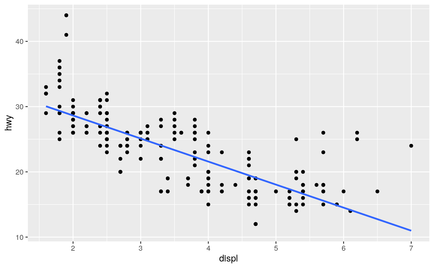
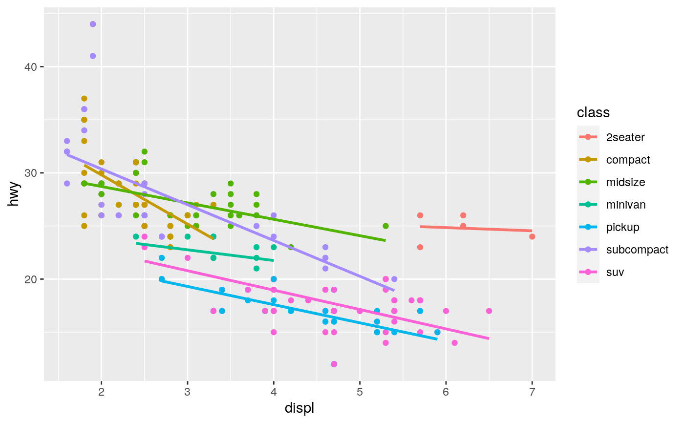
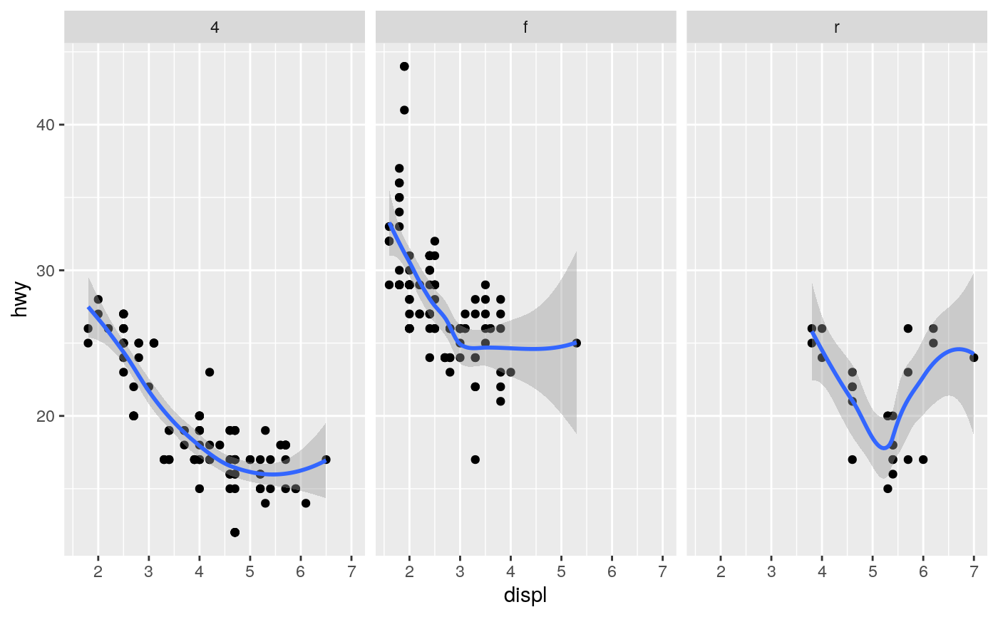
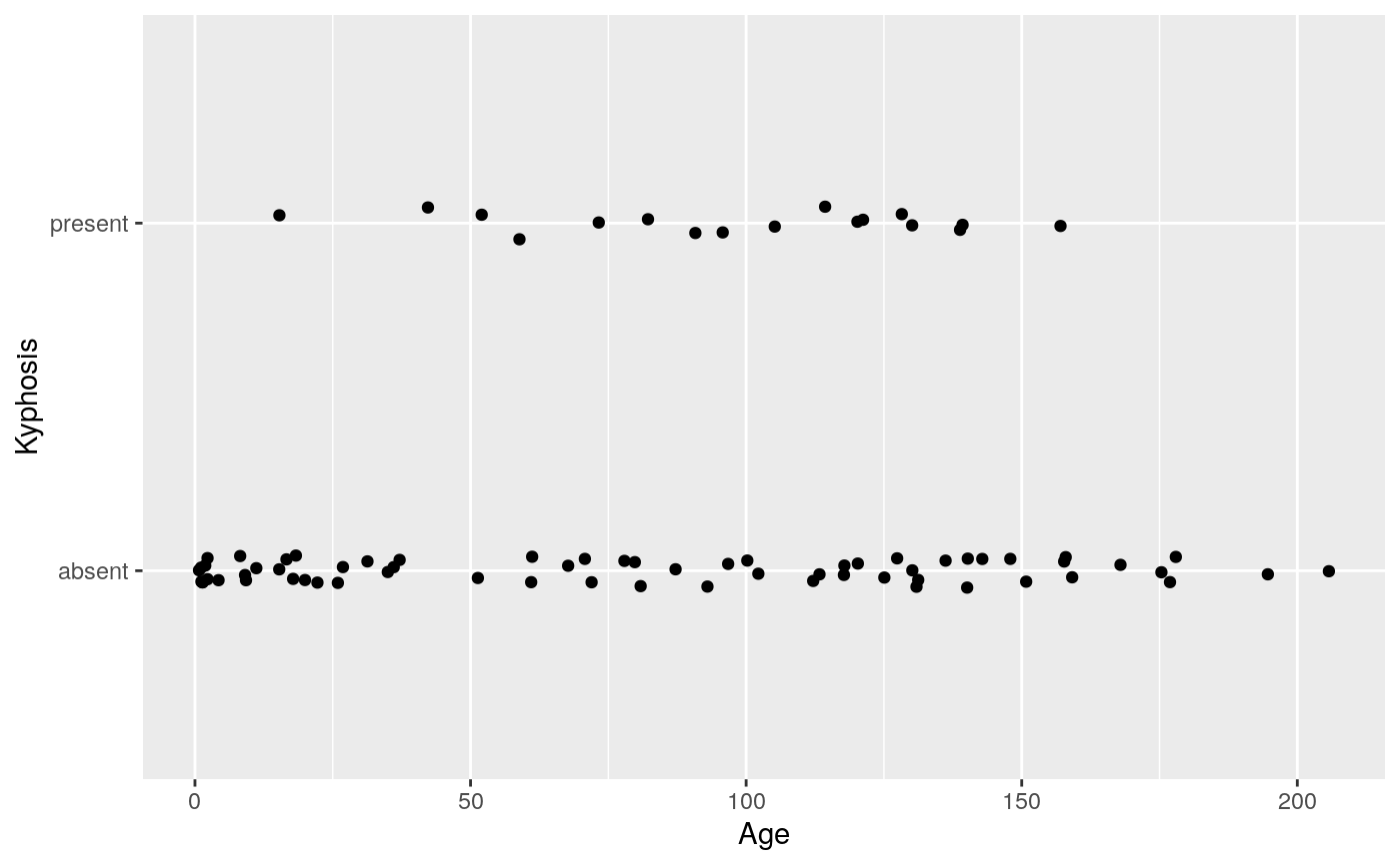
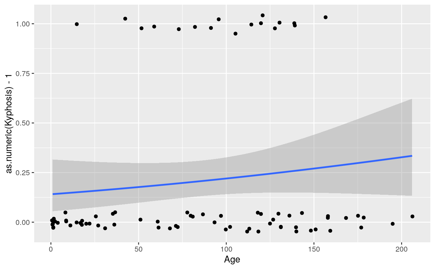
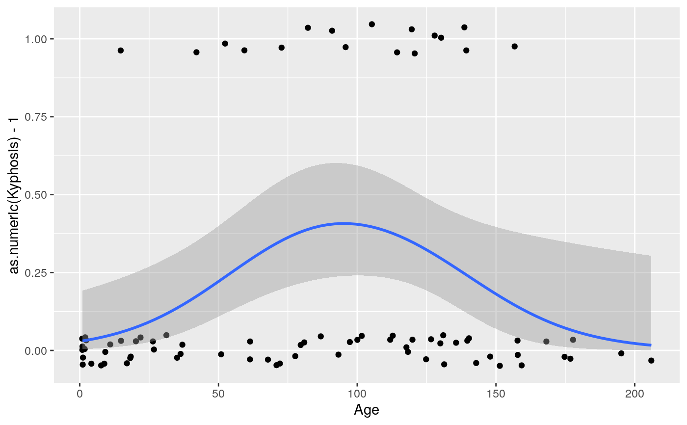
# If you need the fitting to be done along the y-axis set the orientation
ggplot(mpg, aes(displ, hwy)) +
  geom_point() +
  geom_smooth(orientation = "y")
#> `geom_smooth()` using method = 'loess' and formula 'y ~ x'

# Use span to control the "wiggliness" of the default loess smoother.
# The span is the fraction of points used to fit each local regression:
# small numbers make a wigglier curve, larger numbers make a smoother curve.
ggplot(mpg, aes(displ, hwy)) +
  geom_point() +
  geom_smooth(span = 0.3)
#> `geom_smooth()` using method = 'loess' and formula 'y ~ x'

# Instead of a loess smooth, you can use any other modelling function:
ggplot(mpg, aes(displ, hwy)) +
  geom_point() +
  geom_smooth(method = lm, se = FALSE)
#> `geom_smooth()` using formula 'y ~ x'

ggplot(mpg, aes(displ, hwy)) +
  geom_point() +
  geom_smooth(method = lm, formula = y ~ splines::bs(x, 3), se = FALSE)

# Smooths are automatically fit to each group (defined by categorical
# aesthetics or the group aesthetic) and for each facet.

ggplot(mpg, aes(displ, hwy, colour = class)) +
  geom_point() +
  geom_smooth(se = FALSE, method = lm)
#> `geom_smooth()` using formula 'y ~ x'
ggplot(mpg, aes(displ, hwy)) +
  geom_point() +
  geom_smooth(span = 0.8) +
  facet_wrap(~drv)
#> `geom_smooth()` using method = 'loess' and formula 'y ~ x'

# \donttest{
binomial_smooth <- function(...) {
  geom_smooth(method = "glm", method.args = list(family = "binomial"), ...)
}
# To fit a logistic regression, you need to coerce the values to
# a numeric vector lying between 0 and 1.
ggplot(rpart::kyphosis, aes(Age, Kyphosis)) +
  geom_jitter(height = 0.05) +
  binomial_smooth()
#> `geom_smooth()` using formula 'y ~ x'
#> Warning: Computation failed in `stat_smooth()`:
#> y values must be 0 <= y <= 1

ggplot(rpart::kyphosis, aes(Age, as.numeric(Kyphosis) - 1)) +
  geom_jitter(height = 0.05) +
  binomial_smooth()
#> `geom_smooth()` using formula 'y ~ x'

ggplot(rpart::kyphosis, aes(Age, as.numeric(Kyphosis) - 1)) +
  geom_jitter(height = 0.05) +
  binomial_smooth(formula = y ~ splines::ns(x, 2))

# But in this case, it's probably better to fit the model yourself
# so you can exercise more control and see whether or not it's a good model.
# }