Visualise sf objects

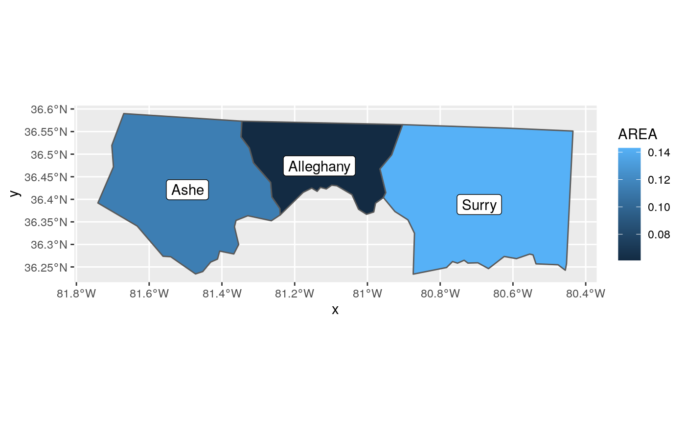
This set of geom, stat, and coord are used to visualise simple feature (sf) objects. For simple plots, you will only need geom_sf() as it uses stat_sf() and adds coord_sf() for you. geom_sf() is an unusual geom because it will draw different geometric objects depending on what simple features are present in the data: you can get points, lines, or polygons. For text and labels, you can use geom_sf_text() and geom_sf_label().

coord_sf(
  xlim = NULL,
  ylim = NULL,
  expand = TRUE,
  crs = NULL,
  datum = sf::st_crs(4326),
  label_graticule = waiver(),
  label_axes = waiver(),
  ndiscr = 100,
  default = FALSE,
  clip = "on"
)

geom_sf(
  mapping = aes(),
  data = NULL,
  stat = "sf",
  position = "identity",
  na.rm = FALSE,
  show.legend = NA,
  inherit.aes = TRUE,
  ...
)

geom_sf_label(
  mapping = aes(),
  data = NULL,
  stat = "sf_coordinates",
  position = "identity",
  ...,
  parse = FALSE,
  nudge_x = 0,
  nudge_y = 0,
  label.padding = unit(0.25, "lines"),
  label.r = unit(0.15, "lines"),
  label.size = 0.25,
  na.rm = FALSE,
  show.legend = NA,
  inherit.aes = TRUE,
  fun.geometry = NULL
)

geom_sf_text(
  mapping = aes(),
  data = NULL,
  stat = "sf_coordinates",
  position = "identity",
  ...,
  parse = FALSE,
  nudge_x = 0,
  nudge_y = 0,
  check_overlap = FALSE,
  na.rm = FALSE,
  show.legend = NA,
  inherit.aes = TRUE,
  fun.geometry = NULL
)

stat_sf(
  mapping = NULL,
  data = NULL,
  geom = "rect",
  position = "identity",
  na.rm = FALSE,
  show.legend = NA,
  inherit.aes = TRUE,
  ...
)

Arguments

xlim	Limits for the x and y axes.
ylim	Limits for the x and y axes.
expand	If `TRUE`, the default, adds a small expansion factor to the limits to ensure that data and axes don't overlap. If `FALSE`, limits are taken exactly from the data or `xlim`/`ylim`.
crs	Use this to select a specific coordinate reference system (CRS). If not specified, will use the CRS defined in the first layer.
datum	CRS that provides datum to use when generating graticules
label_graticule	Character vector indicating which graticule lines should be labeled where. Meridians run north-south, and the letters `"N"` and `"S"` indicate that they should be labeled on their north or south end points, respectively. Parallels run east-west, and the letters `"E"` and `"W"` indicate that they should be labeled on their east or west end points, respectively. Thus, `label_graticule = "SW"` would label meridians at their south end and parallels at their west end, whereas `label_graticule = "EW"` would label parallels at both ends and meridians not at all. Because meridians and parallels can in general intersect with any side of the plot panel, for any choice of `label_graticule` labels are not guaranteed to reside on only one particular side of the plot panel. This parameter can be used alone or in combination with `label_axes`.
label_axes	Character vector or named list of character values specifying which graticule lines (meridians or parallels) should be labeled on which side of the plot. Meridians are indicated by `"E"` (for East) and parallels by `"N"` (for North). Default is `"--EN"`, which specifies (clockwise from the top) no labels on the top, none on the right, meridians on the bottom, and parallels on the left. Alternatively, this setting could have been specified with `list(bottom = "E", left = "N")`. This parameter can be used alone or in combination with `label_graticule`.
ndiscr	number of segments to use for discretising graticule lines; try increasing this when graticules look unexpected
default	Is this the default coordinate system? If `FALSE` (the default), then replacing this coordinate system with another one creates a message alerting the user that the coordinate system is being replaced. If `TRUE`, that warning is suppressed.
clip	Should drawing be clipped to the extent of the plot panel? A setting of `"on"` (the default) means yes, and a setting of `"off"` means no. In most cases, the default of `"on"` should not be changed, as setting `clip = "off"` can cause unexpected results. It allows drawing of data points anywhere on the plot, including in the plot margins. If limits are set via `xlim` and `ylim` and some data points fall outside those limits, then those data points may show up in places such as the axes, the legend, the plot title, or the plot margins.
mapping	Set of aesthetic mappings created by `aes()` or `aes_()`. If specified and `inherit.aes = TRUE` (the default), it is combined with the default mapping at the top level of the plot. You must supply `mapping` if there is no plot mapping.
data	The data to be displayed in this layer. There are three options: If `NULL`, the default, the data is inherited from the plot data as specified in the call to `ggplot()`. A `data.frame`, or other object, will override the plot data. All objects will be fortified to produce a data frame. See `fortify()` for which variables will be created. A `function` will be called with a single argument, the plot data. The return value must be a `data.frame`, and will be used as the layer data. A `function` can be created from a `formula` (e.g. `~ head(.x, 10)`).
stat	The statistical transformation to use on the data for this layer, as a string.
position	Position adjustment, either as a string, or the result of a call to a position adjustment function.
na.rm	If `FALSE`, the default, missing values are removed with a warning. If `TRUE`, missing values are silently removed.
show.legend	logical. Should this layer be included in the legends? `NA`, the default, includes if any aesthetics are mapped. `FALSE` never includes, and `TRUE` always includes. You can also set this to one of "polygon", "line", and "point" to override the default legend.
inherit.aes	If `FALSE`, overrides the default aesthetics, rather than combining with them. This is most useful for helper functions that define both data and aesthetics and shouldn't inherit behaviour from the default plot specification, e.g. `borders()`.
...	Other arguments passed on to `layer()`. These are often aesthetics, used to set an aesthetic to a fixed value, like `colour = "red"` or `size = 3`. They may also be parameters to the paired geom/stat.
parse	If `TRUE`, the labels will be parsed into expressions and displayed as described in `?plotmath`.
nudge_x	Horizontal and vertical adjustment to nudge labels by. Useful for offsetting text from points, particularly on discrete scales.
nudge_y	Horizontal and vertical adjustment to nudge labels by. Useful for offsetting text from points, particularly on discrete scales.
label.padding	Amount of padding around label. Defaults to 0.25 lines.
label.r	Radius of rounded corners. Defaults to 0.15 lines.
label.size	Size of label border, in mm.
fun.geometry	A function that takes a `sfc` object and returns a `sfc_POINT` with the same length as the input. If `NULL`, `function(x) sf::st_point_on_surface(sf::st_zm(x))` will be used. Note that the function may warn about the incorrectness of the result if the data is not projected, but you can ignore this except when you really care about the exact locations.
check_overlap	If `TRUE`, text that overlaps previous text in the same layer will not be plotted.
geom	The geometric object to use display the data

Geometry aesthetic

geom_sf() uses a unique aesthetic: geometry, giving an column of class sfc containing simple features data. There are three ways to supply the geometry aesthetic:

Do nothing: by default geom_sf() assumes it is stored in the geometry column.
Explicitly pass an sf object to the data argument. This will use the primary geometry column, no matter what it's called.
Supply your own using aes(geometry = my_column)

Unlike other aesthetics, geometry will never be inherited from the plot.

CRS

coord_sf() ensures that all layers use a common CRS. You can either specify it using the CRS param, or coord_sf() will take it from the first layer that defines a CRS.

Examples

if (requireNamespace("sf", quietly = TRUE)) {
nc <- sf::st_read(system.file("shape/nc.shp", package = "sf"), quiet = TRUE)
ggplot(nc) +
  geom_sf(aes(fill = AREA))

# If not supplied, coord_sf() will take the CRS from the first layer
# and automatically transform all other layers to use that CRS. This
# ensures that all data will correctly line up
nc_3857 <- sf::st_transform(nc, 3857)
ggplot() +
  geom_sf(data = nc) +
  geom_sf(data = nc_3857, colour = "red", fill = NA)

# Unfortunately if you plot other types of feature you'll need to use
# show.legend to tell ggplot2 what type of legend to use
nc_3857$mid <- sf::st_centroid(nc_3857$geometry)
ggplot(nc_3857) +
  geom_sf(colour = "white") +
  geom_sf(aes(geometry = mid, size = AREA), show.legend = "point")

# You can also use layers with x and y aesthetics: these are
# assumed to already be in the common CRS.
ggplot(nc) +
  geom_sf() +
  annotate("point", x = -80, y = 35, colour = "red", size = 4)

# Thanks to the power of sf, a geom_sf nicely handles varying projections
# setting the aspect ratio correctly.
library(maps)
world1 <- sf::st_as_sf(map('world', plot = FALSE, fill = TRUE))
ggplot() + geom_sf(data = world1)

world2 <- sf::st_transform(
  world1,
  "+proj=laea +y_0=0 +lon_0=155 +lat_0=-90 +ellps=WGS84 +no_defs"
)
ggplot() + geom_sf(data = world2)

# To add labels, use geom_sf_label().
ggplot(nc_3857[1:3, ]) +
   geom_sf(aes(fill = AREA)) +
   geom_sf_label(aes(label = NAME))
}

Arguments

Geometry aesthetic

CRS

See also

Examples