Specify a secondary axis

This function is used in conjunction with a position scale to create a secondary axis, positioned opposite of the primary axis. All secondary axes must be based on a one-to-one transformation of the primary axes.

sec_axis(
  trans = NULL,
  name = waiver(),
  breaks = waiver(),
  labels = waiver(),
  guide = waiver()
)

dup_axis(
  trans = ~.,
  name = derive(),
  breaks = derive(),
  labels = derive(),
  guide = derive()
)

derive()

Arguments

trans	A formula or function of transformation
name	The name of the secondary axis
breaks	One of: NULL for no breaks waiver() for the default breaks computed by the transformation object A numeric vector of positions A function that takes the limits as input and returns breaks as output
labels	One of: NULL for no labels waiver() for the default labels computed by the transformation object A character vector giving labels (must be same length as breaks) A function that takes the breaks as input and returns labels as output
guide	A position guide that will be used to render the axis on the plot. Usually this is guide_axis().

Details

sec_axis is used to create the specifications for a secondary axis. Except for the trans argument any of the arguments can be set to derive() which would result in the secondary axis inheriting the settings from the primary axis.

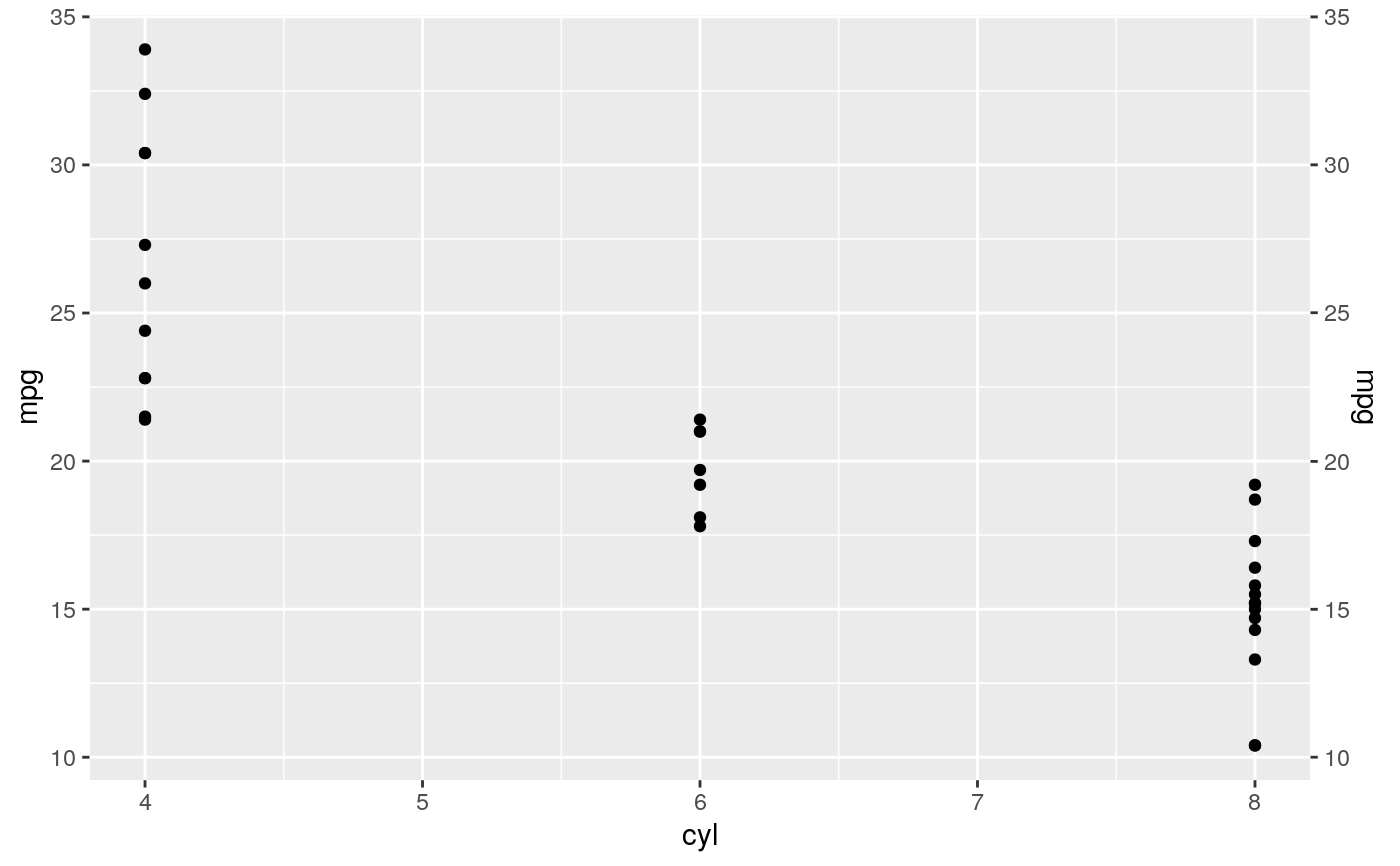
dup_axis is provide as a shorthand for creating a secondary axis that is a duplication of the primary axis, effectively mirroring the primary axis.

As of v3.1, date and datetime scales have limited secondary axis capabilities. Unlike other continuous scales, secondary axis transformations for date and datetime scales must respect their primary POSIX data structure. This means they may only be transformed via addition or subtraction, e.g. ~ . + hms::hms(days = 8), or ~ . - 8*60*60. Nonlinear transformations will return an error. To produce a time-since-event secondary axis in this context, users may consider adapting secondary axis labels.

Examples

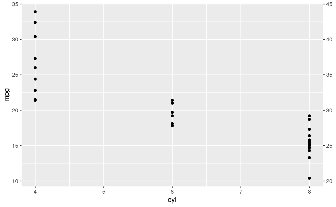
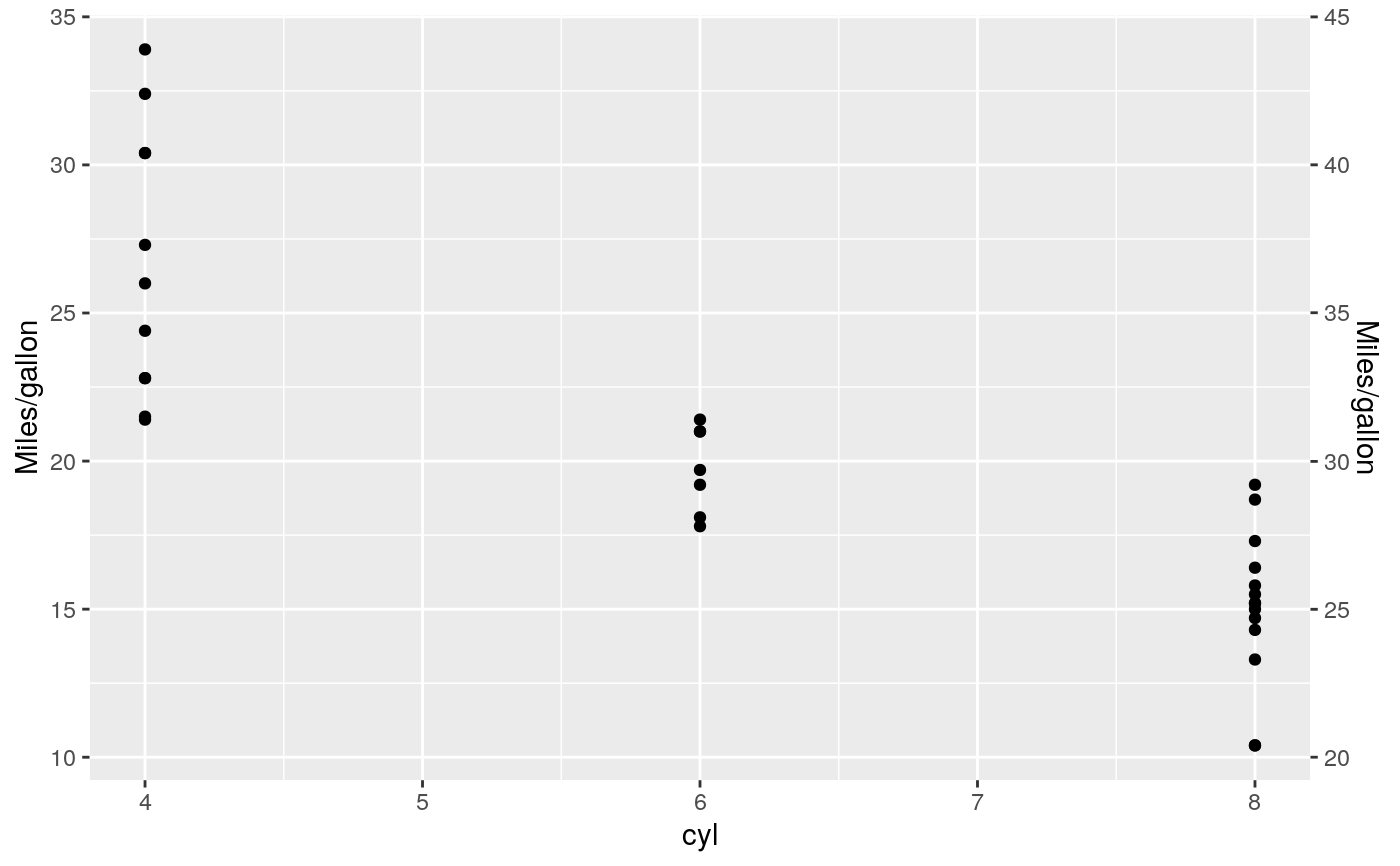
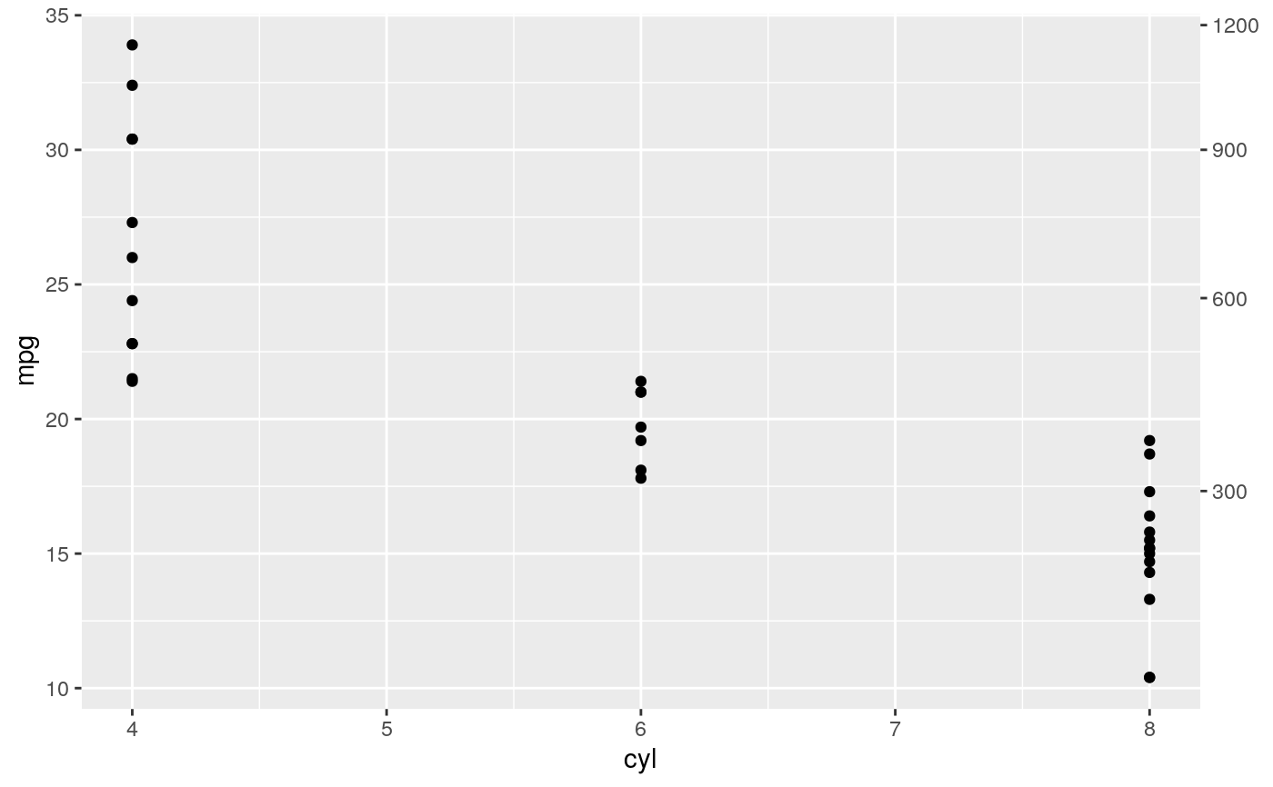
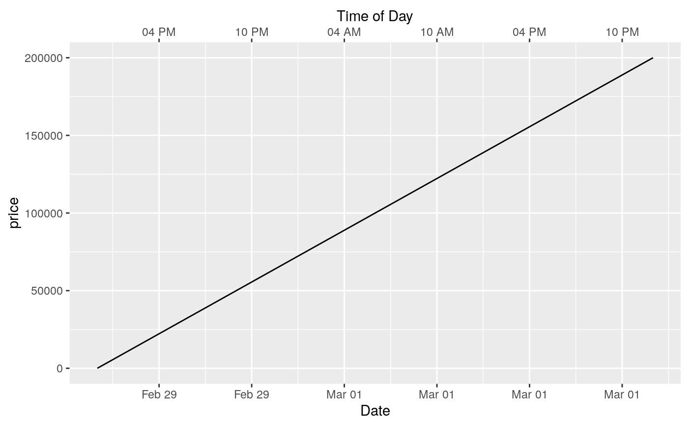
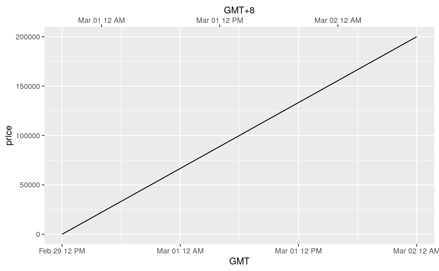
p <- ggplot(mtcars, aes(cyl, mpg)) +
  geom_point()

# Create a simple secondary axis
p + scale_y_continuous(sec.axis = sec_axis(~ . + 10))

# Inherit the name from the primary axis
p + scale_y_continuous("Miles/gallon", sec.axis = sec_axis(~ . + 10, name = derive()))

# Duplicate the primary axis
p + scale_y_continuous(sec.axis = dup_axis())

# You can pass in a formula as a shorthand
p + scale_y_continuous(sec.axis = ~ .^2)

# Secondary axes work for date and datetime scales too:
df <- data.frame(
  dx = seq(as.POSIXct("2012-02-29 12:00:00",
                       tz = "UTC",
                       format = "%Y-%m-%d %H:%M:%S"
  ),
  length.out = 10, by = "4 hour"
  ),
  price = seq(20, 200000, length.out = 10)
 )

# This may useful for labelling different time scales in the same plot
ggplot(df, aes(x = dx, y = price)) + geom_line() +
  scale_x_datetime("Date", date_labels = "%b %d",
  date_breaks = "6 hour",
  sec.axis = dup_axis(name = "Time of Day",
  labels = scales::time_format("%I %p")))

# or to transform axes for different timezones
ggplot(df, aes(x = dx, y = price)) + geom_line() +
  scale_x_datetime("GMT", date_labels = "%b %d %I %p",
  sec.axis = sec_axis(~ . + 8 * 3600, name = "GMT+8",
  labels = scales::time_format("%b %d %I %p")))