Colour related aesthetics: colour, fill, and alpha

These aesthetics parameters change the colour (colour and fill) and the opacity (alpha) of geom elements on a plot. Almost every geom has either colour or fill (or both), as well as can have their alpha modified. Modifying colour on a plot is a useful way to enhance the presentation of data, often especially when a plot graphs more than two variables.

Colour and fill

Colours and fills can be specified in the following ways:

• A name, e.g., "red". R has 657 built-in named colours, which can be listed with grDevices::colors().

• An rgb specification, with a string of the form "#RRGGBB" where each of the pairs RR, GG, BB consists of two hexadecimal digits giving a value in the range 00 to FF. You can optionally make the colour transparent by using the form "#RRGGBBAA".

• An NA, for a completely transparent colour.

Alpha

Alpha refers to the opacity of a geom. Values of alpha range from 0 to 1, with lower values corresponding to more transparent colors.

Alpha can additionally be modified through the colour or fill aesthetic if either aesthetic provides color values using an rgb specification ("#RRGGBBAA"), where AA refers to transparency values.

See also

• Other options for modifying colour: scale_colour_brewer(), scale_colour_gradient(), scale_colour_grey(), scale_colour_hue(), scale_colour_identity(), scale_colour_manual(), scale_colour_viridis_d()

• Other options for modifying fill: scale_fill_brewer(), scale_fill_gradient(), scale_fill_grey(), scale_fill_hue(), scale_fill_identity(), scale_fill_manual(), scale_fill_viridis_d()

• Other options for modifying alpha: scale_alpha()

• Run vignette("ggplot2-specs") to see an overview of other aesthestics that can be modified.

Examples

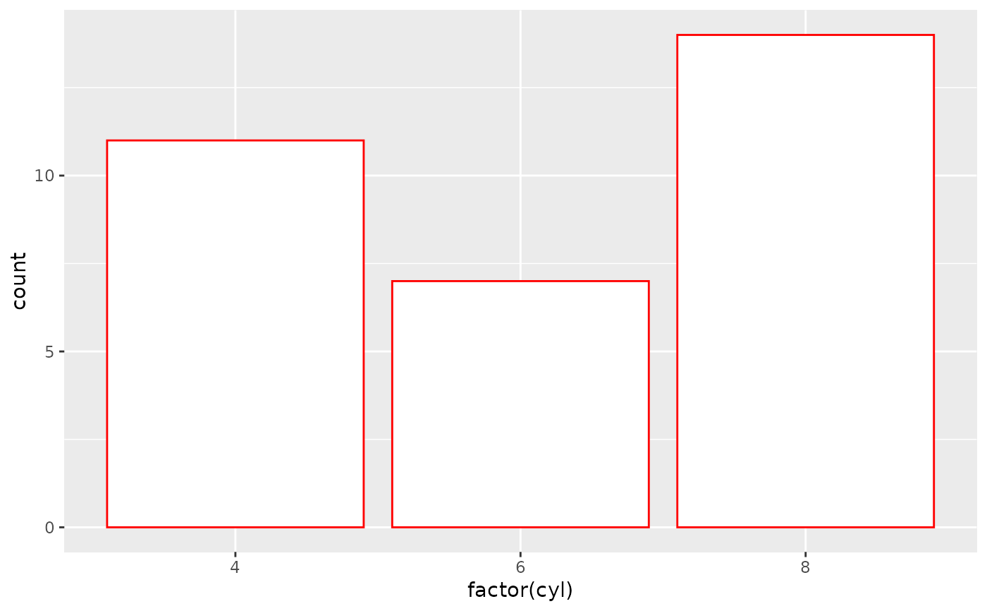
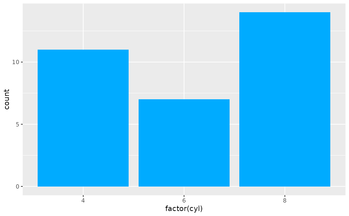
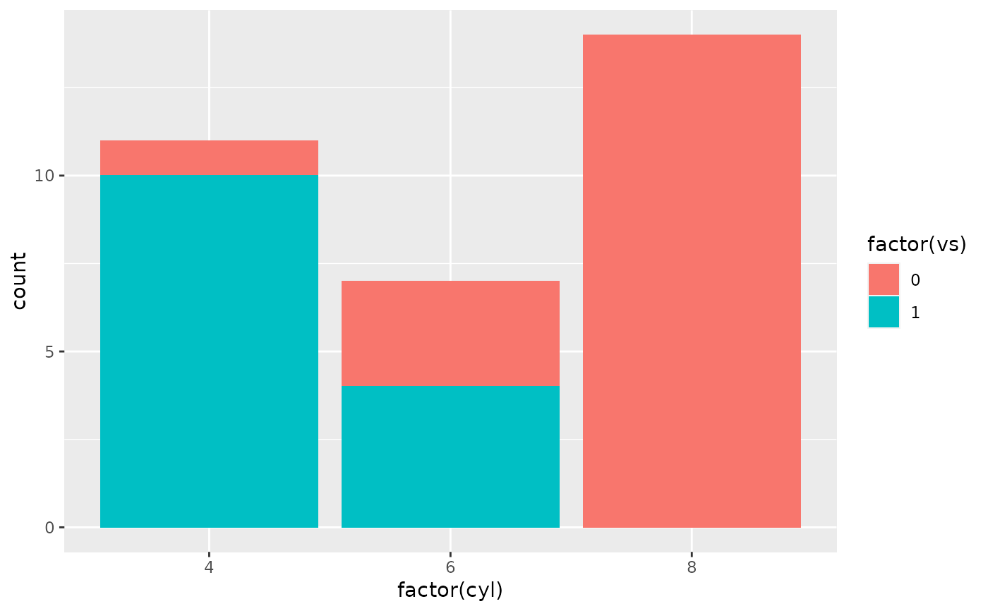
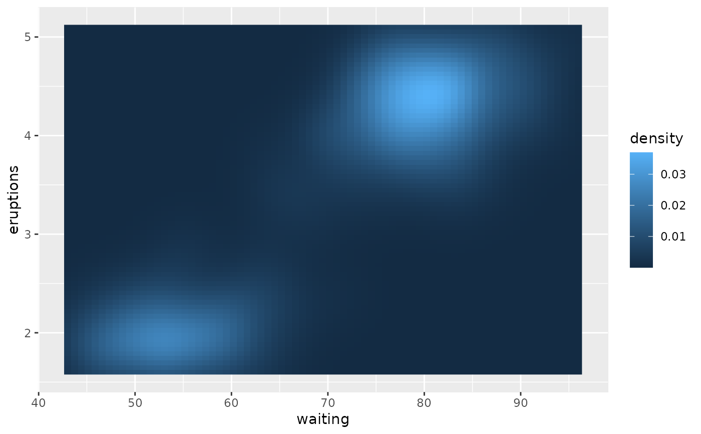
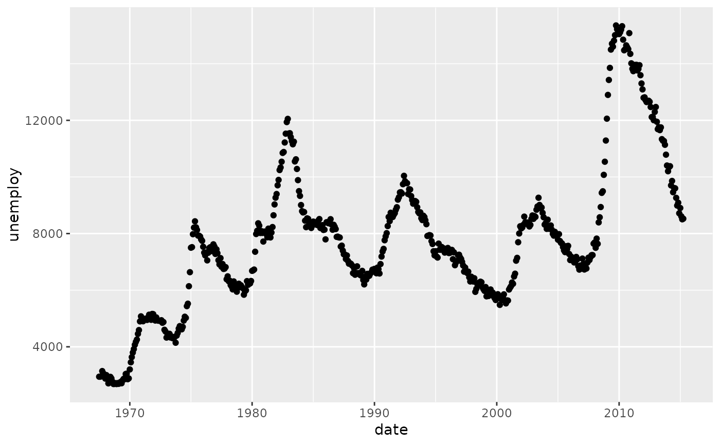
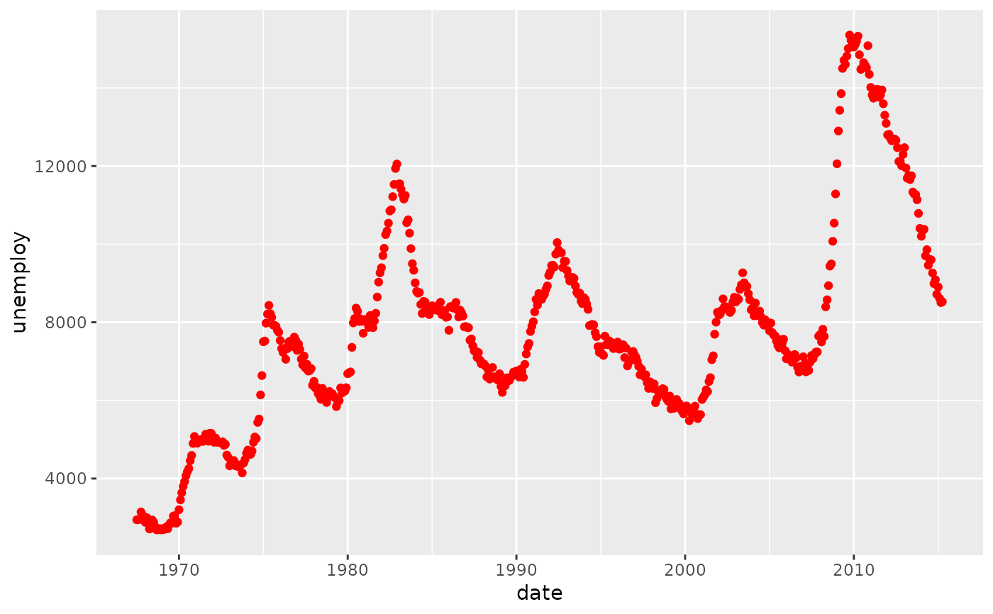
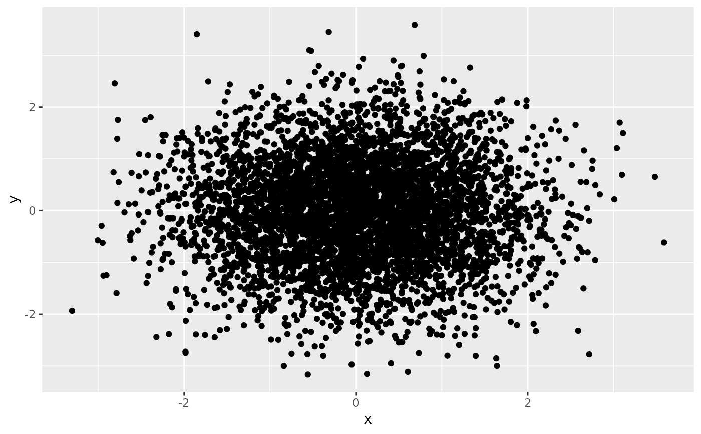
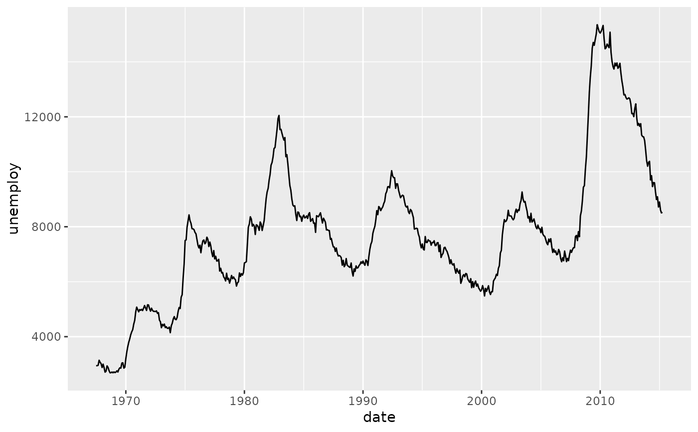
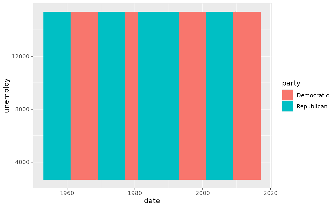
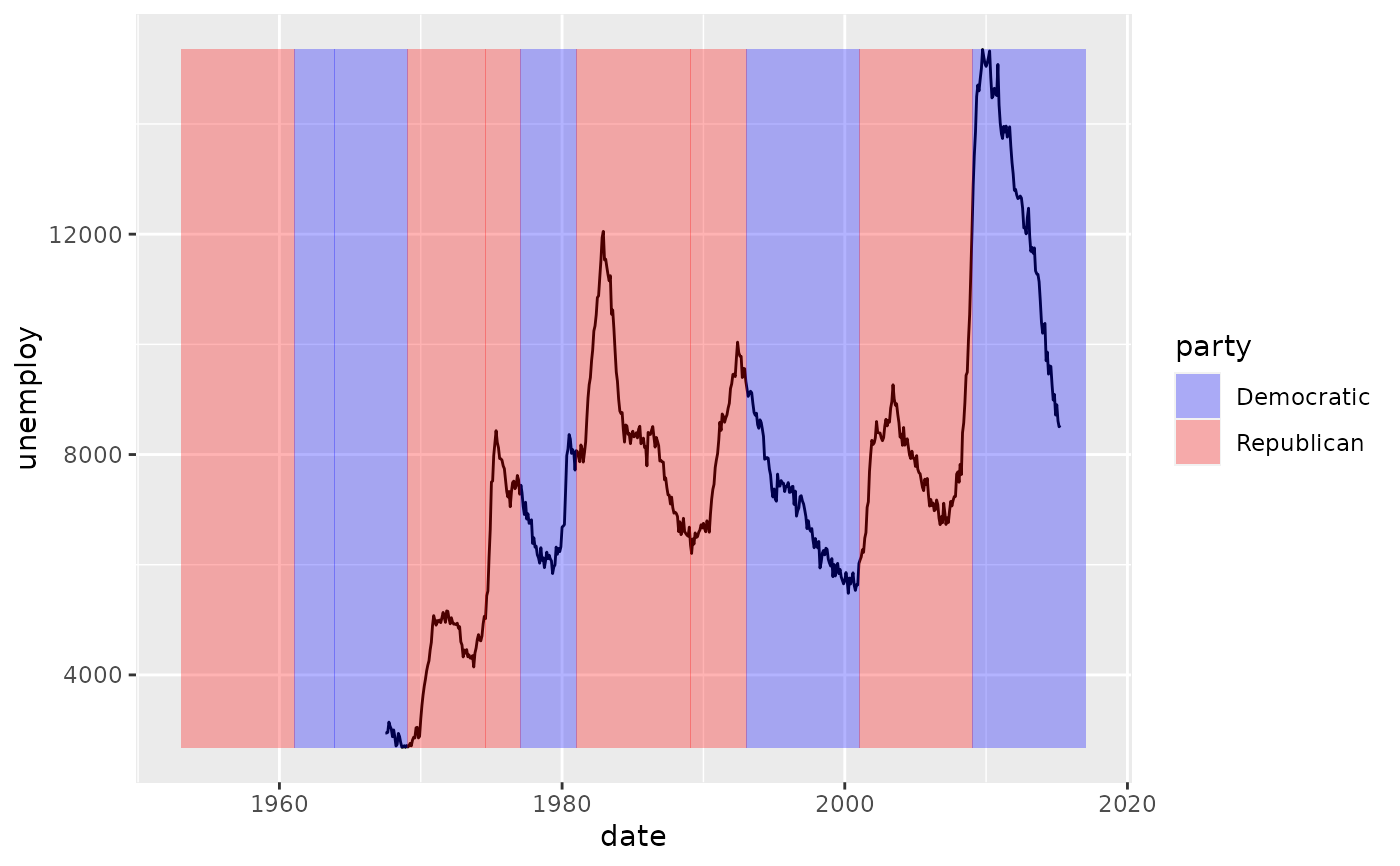
# \donttest{

# Bar chart example
p <- ggplot(mtcars, aes(factor(cyl)))
# Default plotting
p + geom_bar()
# To change the interior colouring use fill aesthetic
p + geom_bar(fill = "red")
# Compare with the colour aesthetic which changes just the bar outline
p + geom_bar(colour = "red")
# Combining both, you can see the changes more clearly
p + geom_bar(fill = "white", colour = "red")
# Both colour and fill can take an rgb specification.
p + geom_bar(fill = "#00abff")
# Use NA for a completely transparent colour.
p + geom_bar(fill = NA, colour = "#00abff")

# Colouring scales differ depending on whether a discrete or
# continuous variable is being mapped. For example, when mapping
# fill to a factor variable, a discrete colour scale is used.
ggplot(mtcars, aes(factor(cyl), fill = factor(vs))) + geom_bar()

# When mapping fill to continuous variable a continuous colour
# scale is used.
ggplot(faithfuld, aes(waiting, eruptions)) +
  geom_raster(aes(fill = density))

# Some geoms only use the colour aesthetic but not the fill
# aesthetic (e.g. geom_point() or geom_line()).
p <- ggplot(economics, aes(x = date, y = unemploy))
p + geom_line()
p + geom_line(colour = "green")
p + geom_point()
p + geom_point(colour = "red")

# For large datasets with overplotting the alpha
# aesthetic will make the points more transparent.
df <- data.frame(x = rnorm(5000), y = rnorm(5000))
p  <- ggplot(df, aes(x,y))
p + geom_point()
p + geom_point(alpha = 0.5)
p + geom_point(alpha = 1/10)

# Alpha can also be used to add shading.
p <- ggplot(economics, aes(x = date, y = unemploy)) + geom_line()
p
yrng <- range(economics$unemploy)
p <- p +
  geom_rect(
    aes(NULL, NULL, xmin = start, xmax = end, fill = party),
    ymin = yrng[1], ymax = yrng[2], data = presidential
  )
p
p + scale_fill_manual(values = alpha(c("blue", "red"), .3))
# }