Calculate Time and Amount of Last Dose • lastdose

Overview

Calculate the time since and amount of the last dose. Additional (ADDL) dosing records are expanded and included in the calculation.

Installation

remotes::install_github("metrumresearchgroup/lastdose")

library(lastdose)
library(tidyverse)
theme_set(theme_bw())

A PK profile

We’ll use this PK profile as an example

file <- system.file("csv/data1.csv", package = "lastdose")

df <- read.csv(file) 

head(df)

.   ID TIME EVID  AMT CMT II ADDL   DV
. 1  1    0    0    0   0  0    0  0.0
. 2  1    0    1 1000   1 24   27  0.0
. 3  1    4    0    0   0  0    0 42.1
. 4  1    8    0    0   0  0    0 35.3
. 5  1   12    0    0   0  0    0 28.9
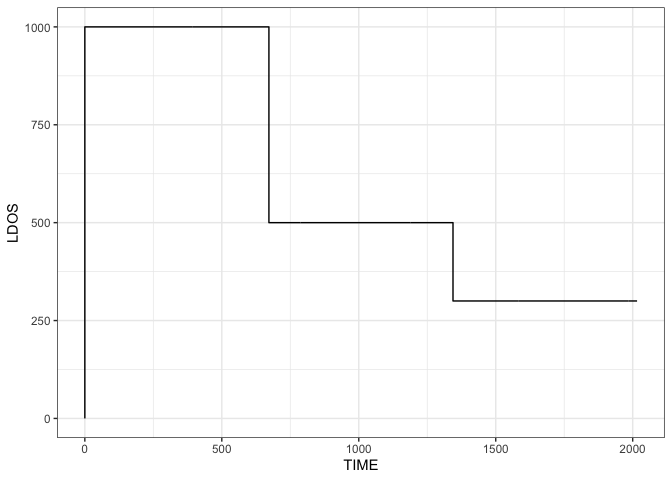
. 6  1   16    0    0   0  0    0 23.6

The dosing runs over 12 weeks and there are 3 epochs, with 3 different doses, most of which are scheduled into the future via ADDL.

df %>% filter(EVID==1) %>% count(TIME,AMT,ADDL)

.   TIME  AMT ADDL n
. 1    0 1000   27 1
. 2  672  500   27 1
. 3 1344  300   27 1

ggplot(df, aes(TIME,DV)) + geom_line() + theme_bw()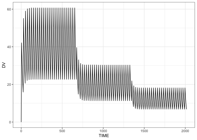

Calculate TAD, TAFD, and LDOS

Use the lastdose() function

df <- lastdose(df)

head(df)

.   ID TIME EVID  AMT CMT II ADDL   DV TAD TAFD LDOS
. 1  1    0    0    0   0  0    0  0.0   0    0    0
. 2  1    0    1 1000   1 24   27  0.0   0    0 1000
. 3  1    4    0    0   0  0    0 42.1   4    4 1000
. 4  1    8    0    0   0  0    0 35.3   8    8 1000
. 5  1   12    0    0   0  0    0 28.9  12   12 1000
. 6  1   16    0    0   0  0    0 23.6  16   16 1000

Now we have TAD, TAFD, and LDOS in our data set.

Plot last dose versus time

ggplot(df, aes(TIME,LDOS)) + geom_line()

Plot time after dose versus time

ggplot(df, aes(TIME,TAD)) + geom_line()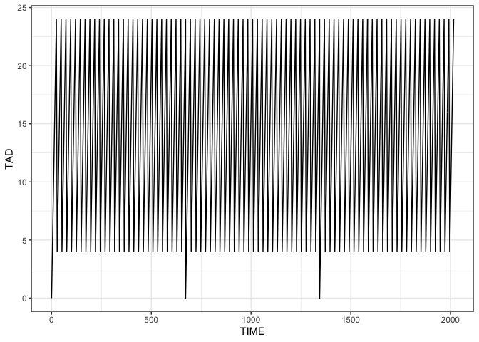

Observations before doses at the same time by default

ggplot(df, aes(TIME,TAD)) + geom_line() + 
  scale_x_continuous(breaks = seq(0,72,4), limits=c(0,72)) + 
  scale_y_continuous(breaks = seq(0,24,4), limits=c(0,24))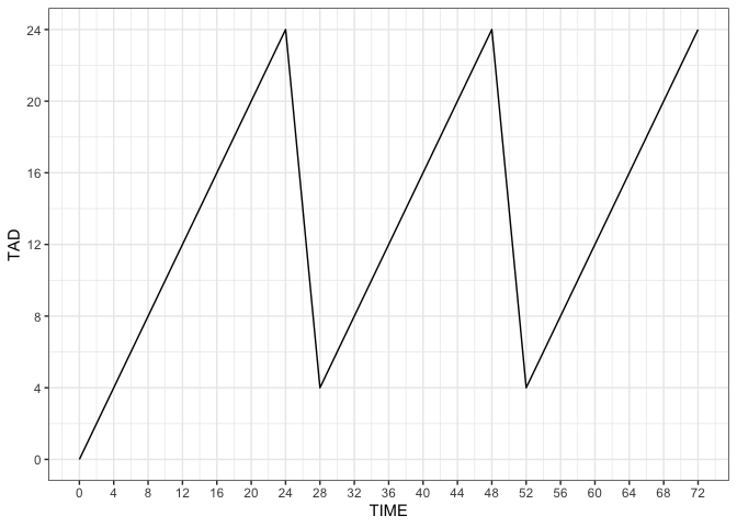

You can also make doses “happen” first

dd <- lastdose(df, addl_ties = "dose_first")

ggplot(dd, aes(TIME,TAD)) + geom_line() + 
  scale_x_continuous(breaks = seq(0,72,4), limits=c(0,72)) + 
  scale_y_continuous(breaks = seq(0,24,4), limits=c(0,24))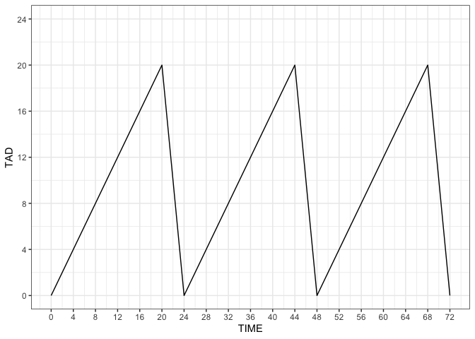

All doses explicit in the data set

df2 <- mrgsolve::realize_addl(df) %>% lastdose()

ggplot(df2, aes(TIME,TAD)) + geom_line() + 
  scale_x_continuous(breaks = seq(0,72,4), limits = c(0,72)) + 
  scale_y_continuous(breaks = seq(0,24,4))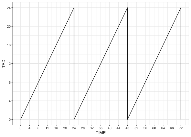

How does it perform on bigger data?

Same setup as the previous profile, but more individuals.

We have 500K rows and 1000 individuals

file <- system.file("csv/data_big.RDS", package = "lastdose")

big <- readRDS(file)

dim(big)

. [1] 508000      8

length(unique(big$ID))

. [1] 1000

Timing result

system.time(x2 <- lastdose(big))

.    user  system elapsed 
.   0.040   0.002   0.041

Compare against the single profile

system.time(x1 <- lastdose(df))

.    user  system elapsed 
.   0.000   0.000   0.001

x3 <- filter(x2, big[["ID"]]==1) %>% as.data.frame()

all.equal(x1,x3)

. [1] TRUE

Observations prior to the first dose

When non-dose records happen prior to the first dose, lastdose calculates the time before the first dose (a negative value) for these records.

file <- system.file("csv/data2.csv", package = "lastdose")

df <- read_csv(file)

lastdose(df) %>% head()

. # A tibble: 6 x 11
.      ID  TIME  EVID   AMT   CMT    II  ADDL    DV   TAD  TAFD  LDOS
.   <dbl> <dbl> <dbl> <dbl> <dbl> <dbl> <dbl> <dbl> <dbl> <dbl> <dbl>
. 1     1     0     0     0     0     0     0   0     -12   -12     0
. 2     1     4     0     0     0     0     0   0      -8    -8     0
. 3     1     8     0     0     0     0     0   0      -4    -4     0
. 4     1    12     0     0     0     0     0   0       0     0     0
. 5     1    12     1  1000     1    24    27   0       0     0  1000
. 6     1    16     0     0     0     0     0  23.6     4     4  1000

The user can alternatively control what happens for these records

lastdose(df, fill = NA_real_, back_calc=FALSE) %>% head()

. # A tibble: 6 x 11
.      ID  TIME  EVID   AMT   CMT    II  ADDL    DV   TAD  TAFD  LDOS
.   <dbl> <dbl> <dbl> <dbl> <dbl> <dbl> <dbl> <dbl> <dbl> <dbl> <dbl>
. 1     1     0     0     0     0     0     0   0      NA    NA     0
. 2     1     4     0     0     0     0     0   0      NA    NA     0
. 3     1     8     0     0     0     0     0   0      NA    NA     0
. 4     1    12     0     0     0     0     0   0      NA    NA     0
. 5     1    12     1  1000     1    24    27   0       0     0  1000
. 6     1    16     0     0     0     0     0  23.6     4     4  1000

More info

See inst/doc/about.md for more details.

lastdose