Set scale limits

This is a shortcut for supplying the limits argument to the individual scales. Note that, by default, any values outside the limits will be replaced with NA.

lims(...)

xlim(...)

ylim(...)

Arguments

...

A name-value pair. The name must be an aesthetic, and the value must be either a length-2 numeric, a character, a factor, or a date/time. A numeric value will create a continuous scale. If the larger value comes first, the scale will be reversed. You can leave one value as NA to compute from the range of the data. A character or factor value will create a discrete scale. A date-time value will create a continuous date/time scale.

See also

For changing x or y axis limits without dropping data observations, see coord_cartesian(). To expand the range of a plot to always include certain values, see expand_limits(). For other types of data, see scale_x_discrete(), scale_x_continuous(), scale_x_date().

Examples

# Zoom into a specified area
ggplot(mtcars, aes(mpg, wt)) +
  geom_point() +
  xlim(15, 20)
#> Warning: Removed 19 rows containing missing values (geom_point).

# reverse scale
ggplot(mtcars, aes(mpg, wt)) +
  geom_point() +
  xlim(20, 15)
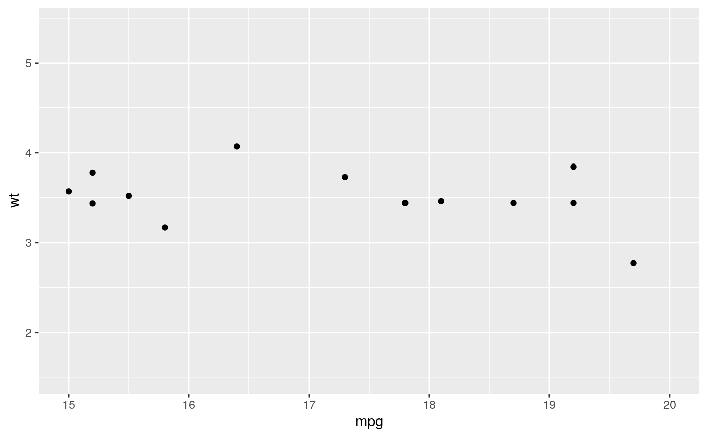
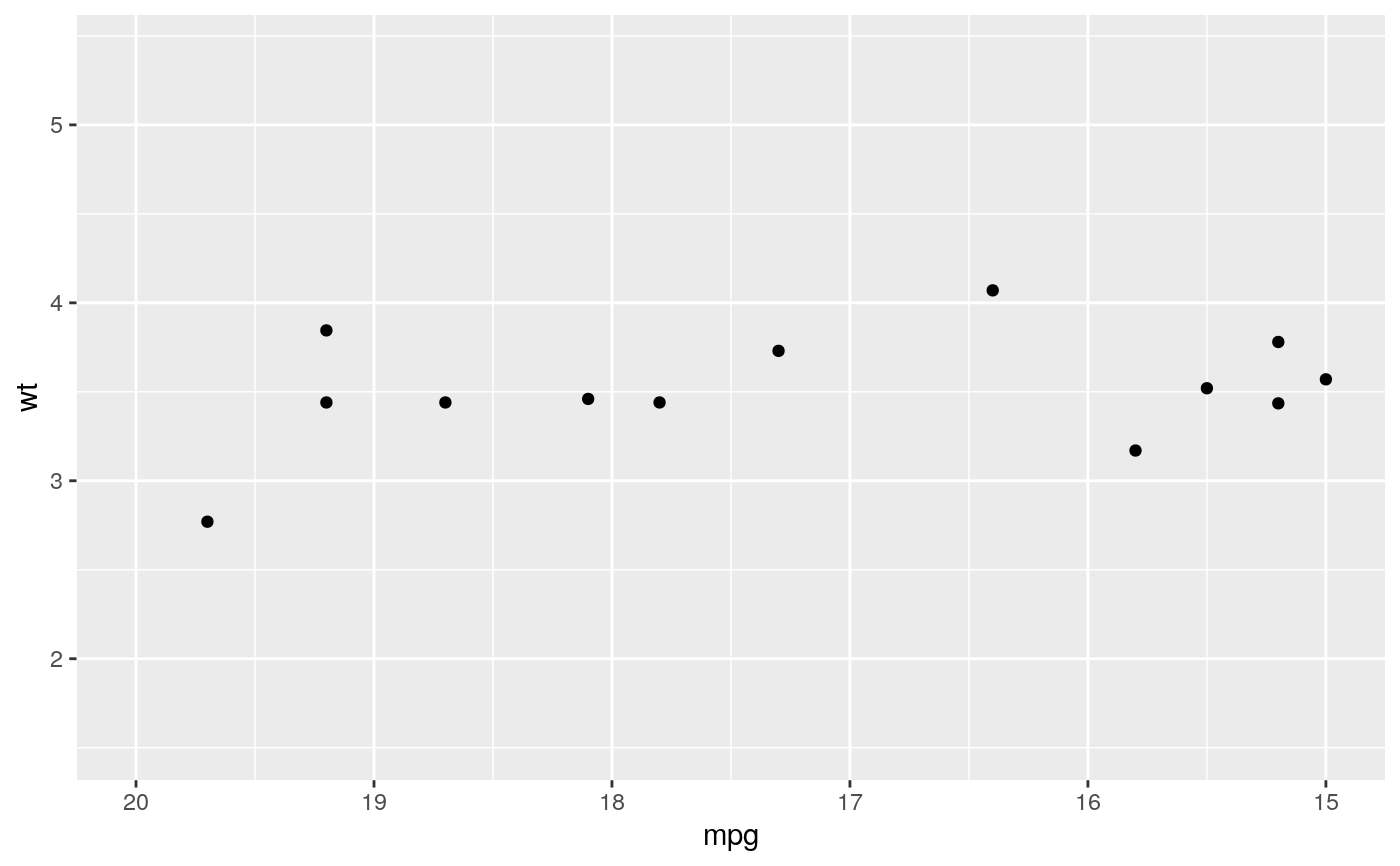
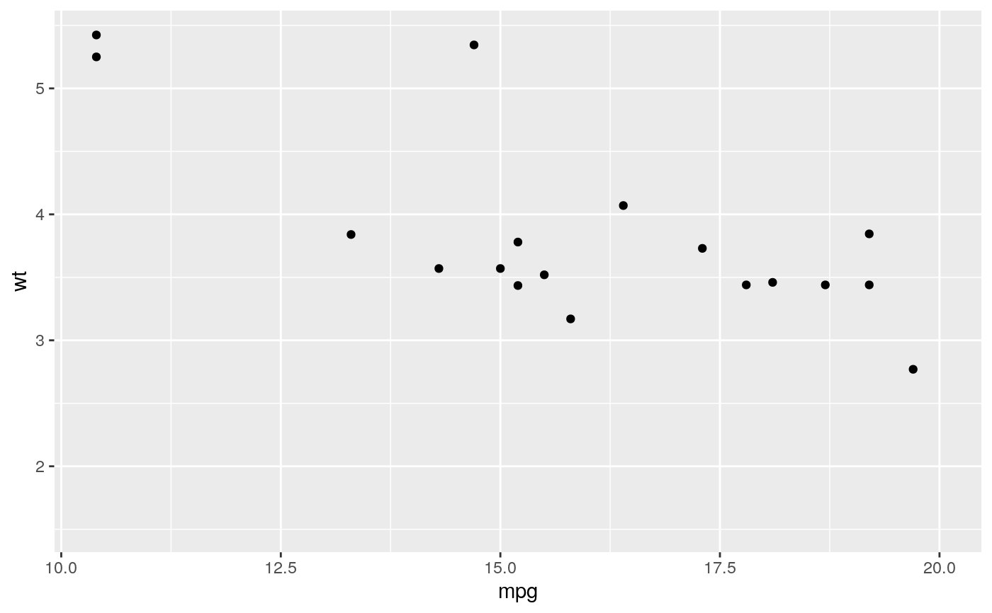
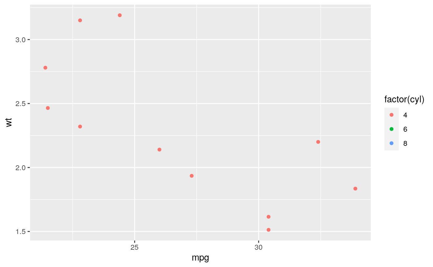
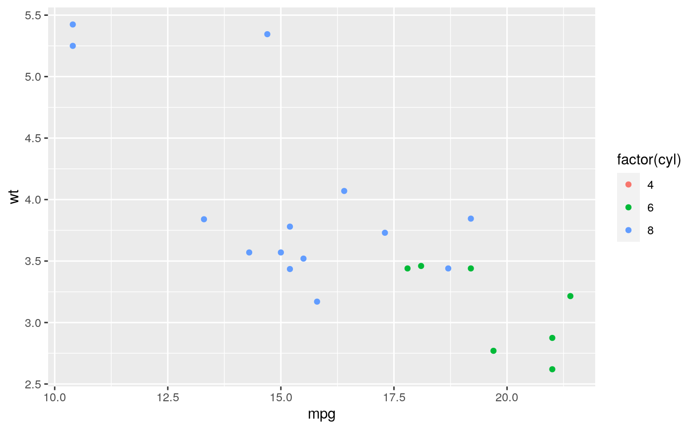
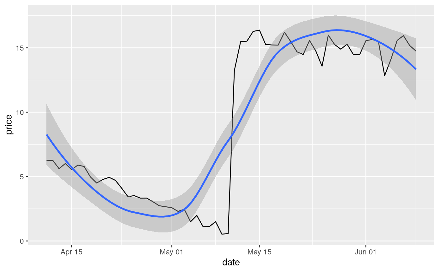
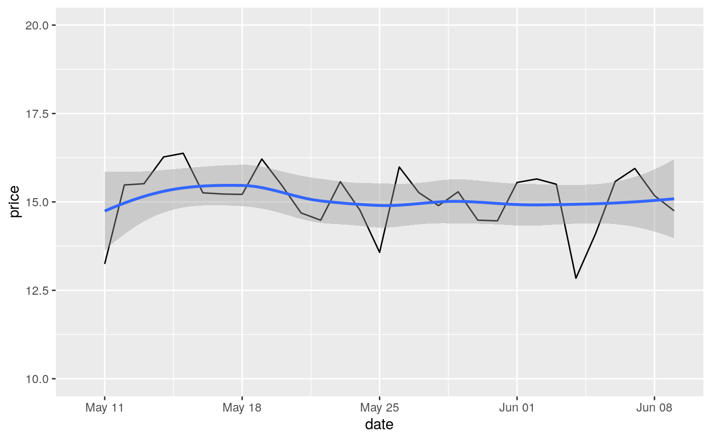
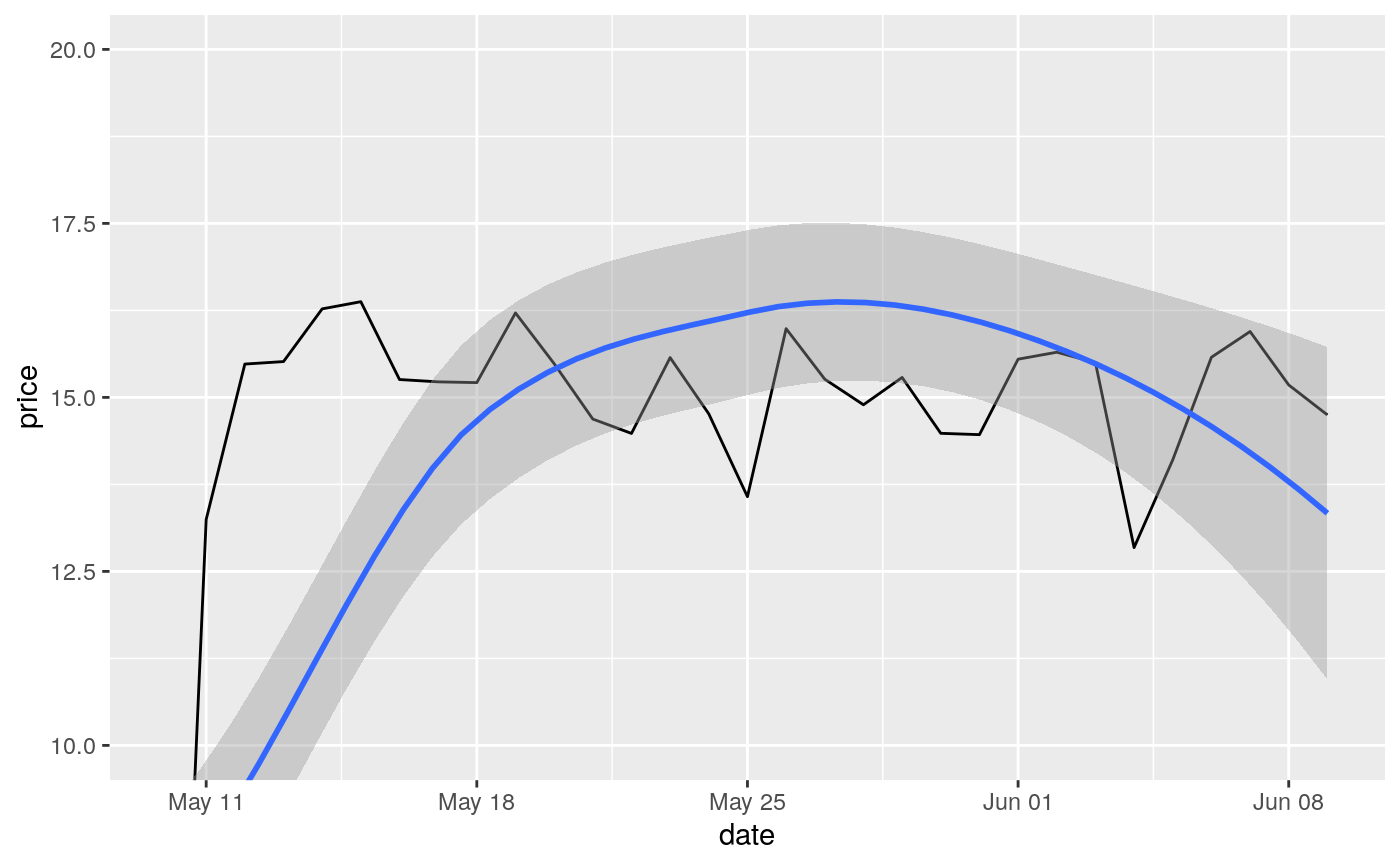
#> Warning: Removed 19 rows containing missing values (geom_point).

# with automatic lower limit
ggplot(mtcars, aes(mpg, wt)) +
  geom_point() +
  xlim(NA, 20)
#> Warning: Removed 14 rows containing missing values (geom_point).

# You can also supply limits that are larger than the data.
# This is useful if you want to match scales across different plots
small <- subset(mtcars, cyl == 4)
big <- subset(mtcars, cyl > 4)

ggplot(small, aes(mpg, wt, colour = factor(cyl))) +
  geom_point() +
  lims(colour = c("4", "6", "8"))

ggplot(big, aes(mpg, wt, colour = factor(cyl))) +
  geom_point() +
  lims(colour = c("4", "6", "8"))

# There are two ways of setting the axis limits: with limits or
# with coordinate systems. They work in two rather different ways.

last_month <- Sys.Date() - 0:59
df <- data.frame(
  date = last_month,
  price = c(rnorm(30, mean = 15), runif(30) + 0.2 * (1:30))
)

p <- ggplot(df, aes(date, price)) +
  geom_line() +
  stat_smooth()

p
#> `geom_smooth()` using method = 'loess' and formula 'y ~ x'

# Setting the limits with the scale discards all data outside the range.
p + lims(x= c(Sys.Date() - 30, NA), y = c(10, 20))
#> `geom_smooth()` using method = 'loess' and formula 'y ~ x'
#> Warning: Removed 30 rows containing non-finite values (stat_smooth).
#> Warning: Removed 30 row(s) containing missing values (geom_path).

# For changing x or y axis limits **without** dropping data
# observations use [coord_cartesian()]. Setting the limits on the
# coordinate system performs a visual zoom.
p + coord_cartesian(xlim =c(Sys.Date() - 30, NA), ylim = c(10, 20))
#> `geom_smooth()` using method = 'loess' and formula 'y ~ x'