Position related aesthetics: x, y, xmin, xmax, ymin, ymax, xend, yend
Source:R/aes-position.r
aes_position.RdThe following aesthetics can be used to specify the position of elements:
x, y, xmin, xmax, ymin, ymax, xend, yend.
Details
x and y define the locations of points or of positions along a line
or path.
x, y and xend, yend define the starting and ending points of
segment and curve geometries.
xmin, xmax, ymin and ymax can be used to specify the position of
annotations and to represent rectangular areas.
See also
Geoms that commonly use these aesthetics:
geom_crossbar(),geom_curve(),geom_errorbar(),geom_line(),geom_linerange(),geom_path(),geom_point(),geom_pointrange(),geom_rect(),geom_segment()See also
annotate()for placing annotations.
Examples
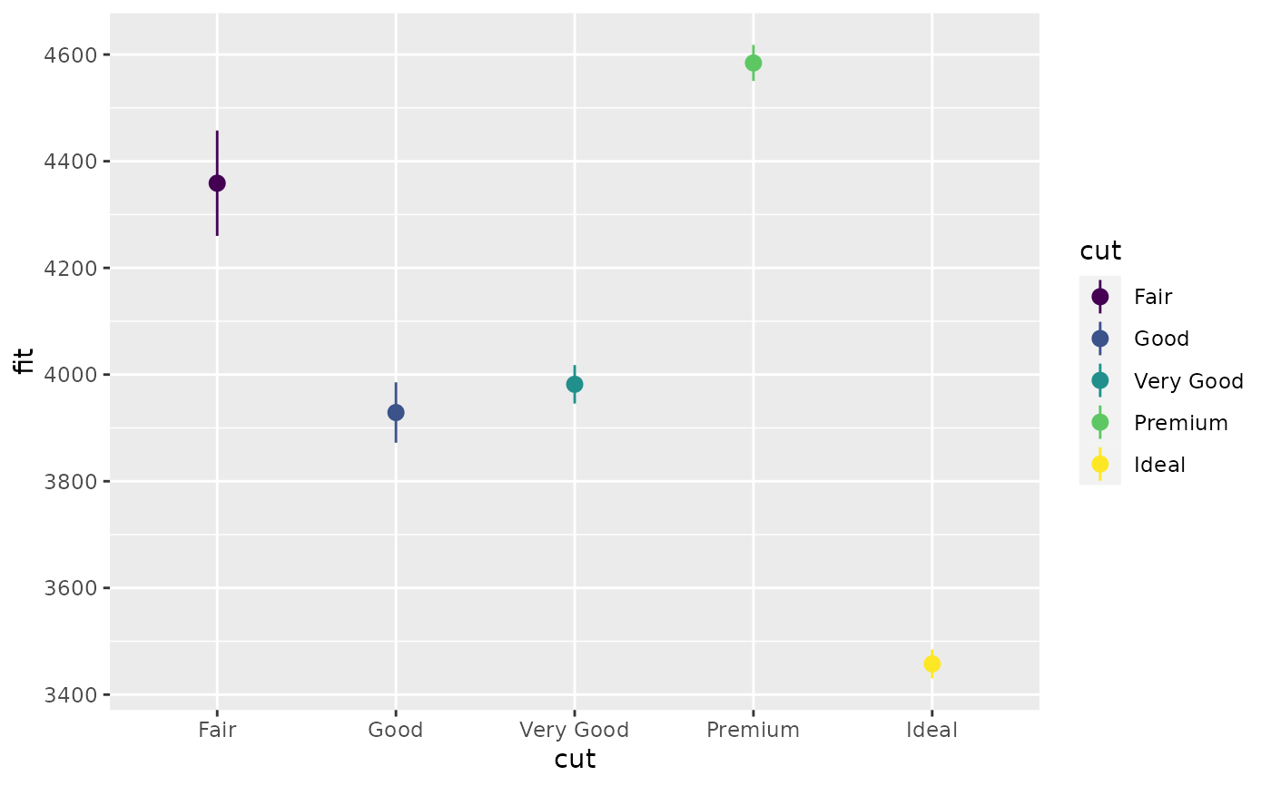
# Generate data: means and standard errors of means for prices
# for each type of cut
dmod <- lm(price ~ cut, data = diamonds)
cut <- unique(diamonds$cut)
cuts_df <- data.frame(
cut,
predict(dmod, data.frame(cut), se = TRUE)[c("fit", "se.fit")]
)
ggplot(cuts_df) +
aes(
x = cut,
y = fit,
ymin = fit - se.fit,
ymax = fit + se.fit,
colour = cut
) +
geom_pointrange()
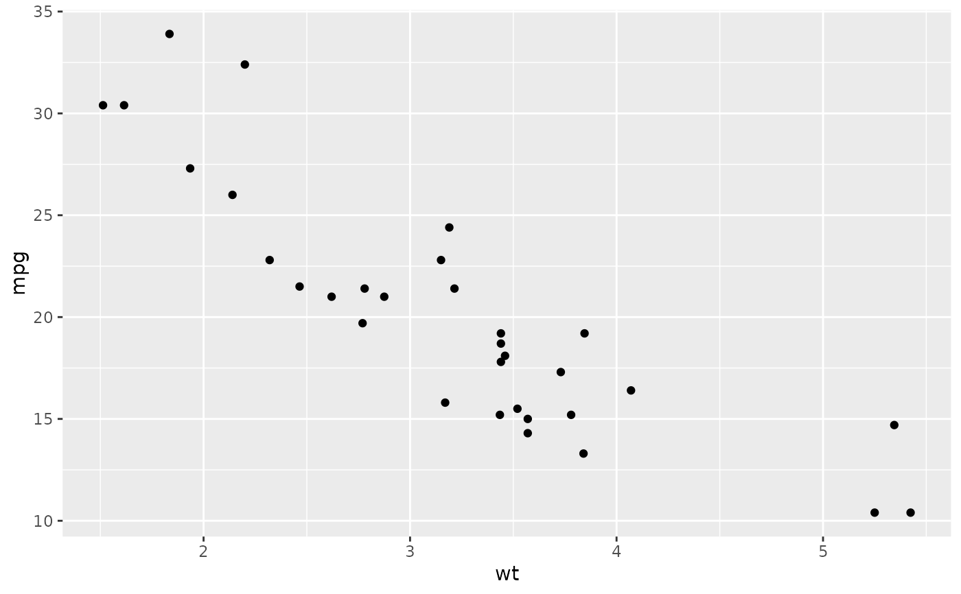
 # Using annotate
p <- ggplot(mtcars, aes(x = wt, y = mpg)) + geom_point()
p
# Using annotate
p <- ggplot(mtcars, aes(x = wt, y = mpg)) + geom_point()
p
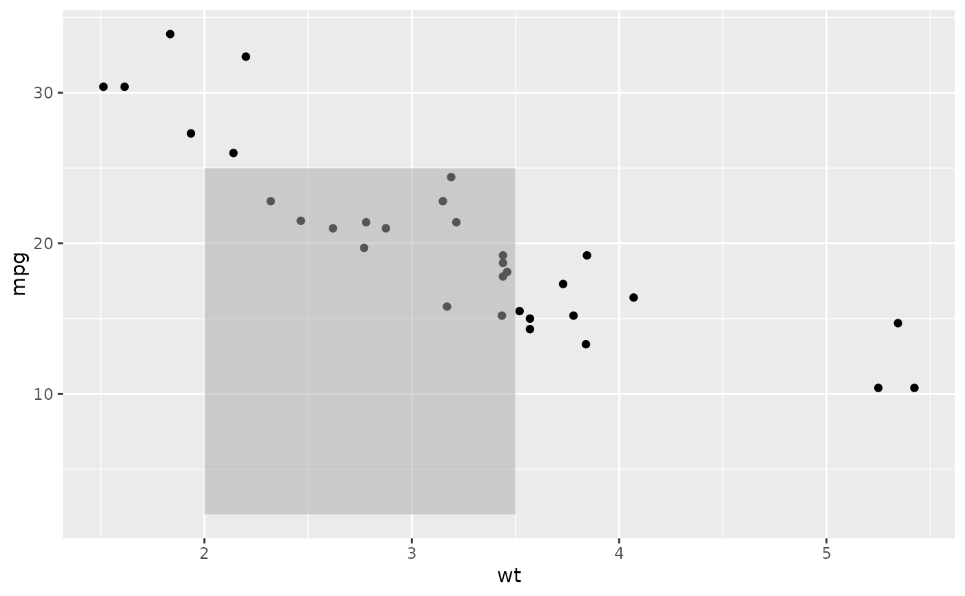
 p + annotate(
"rect", xmin = 2, xmax = 3.5, ymin = 2, ymax = 25,
fill = "dark grey", alpha = .5
)
p + annotate(
"rect", xmin = 2, xmax = 3.5, ymin = 2, ymax = 25,
fill = "dark grey", alpha = .5
)
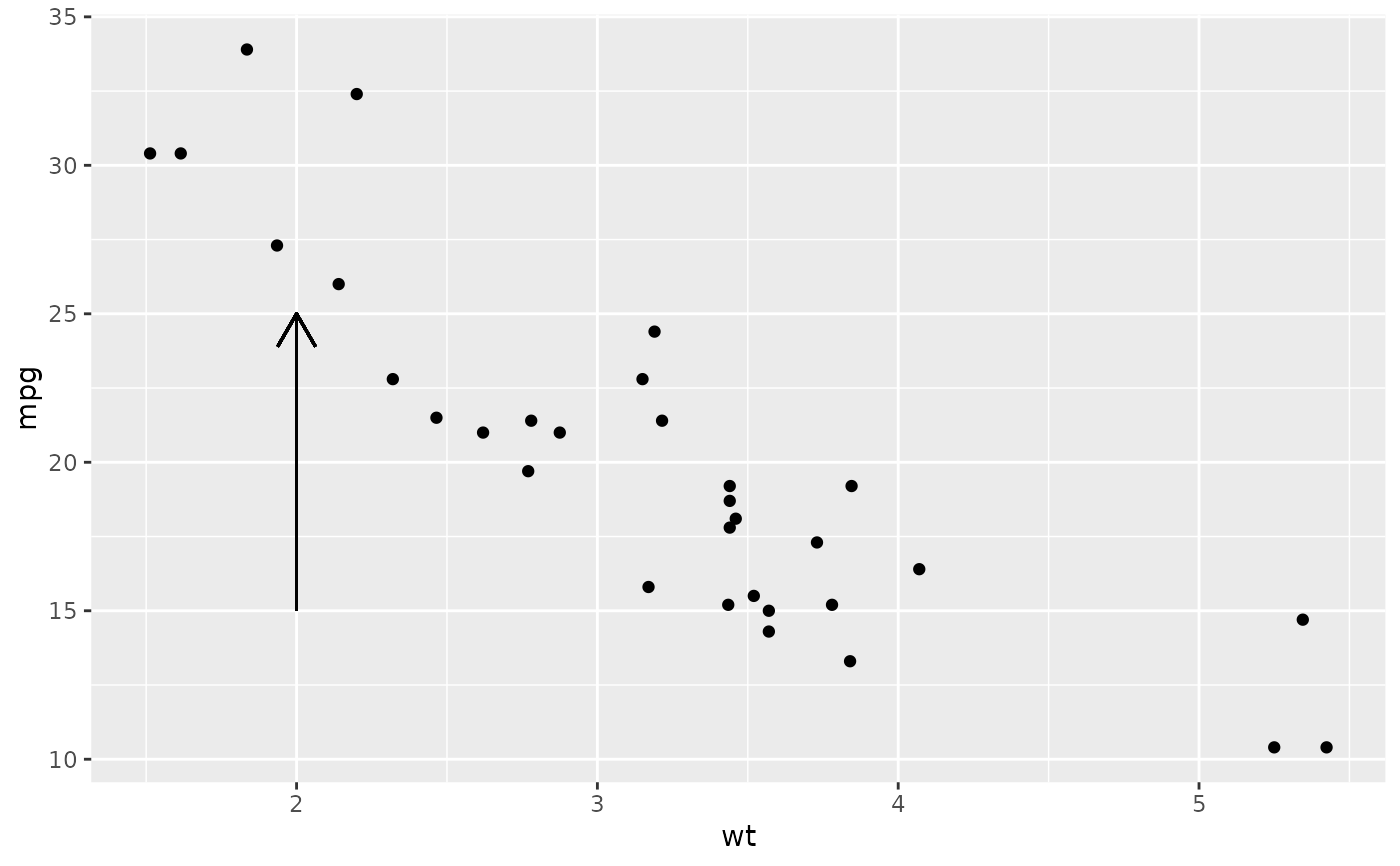
 # Geom_segment examples
p + geom_segment(
aes(x = 2, y = 15, xend = 2, yend = 25),
arrow = arrow(length = unit(0.5, "cm"))
)
# Geom_segment examples
p + geom_segment(
aes(x = 2, y = 15, xend = 2, yend = 25),
arrow = arrow(length = unit(0.5, "cm"))
)
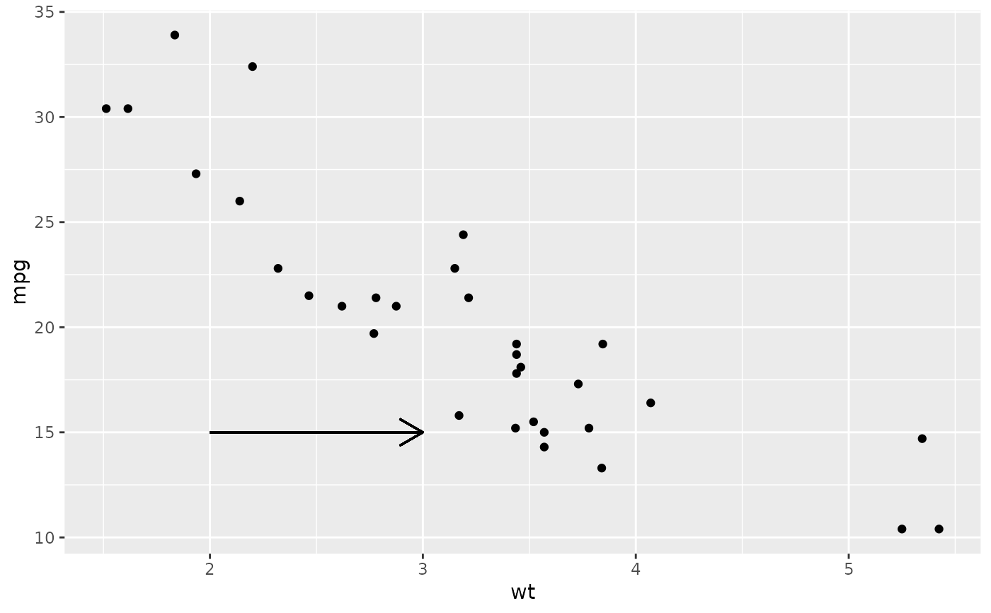
 p + geom_segment(
aes(x = 2, y = 15, xend = 3, yend = 15),
arrow = arrow(length = unit(0.5, "cm"))
)
p + geom_segment(
aes(x = 2, y = 15, xend = 3, yend = 15),
arrow = arrow(length = unit(0.5, "cm"))
)
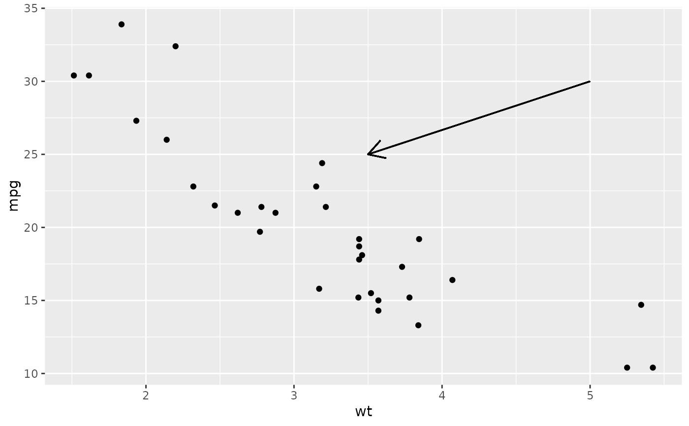
 p + geom_segment(
aes(x = 5, y = 30, xend = 3.5, yend = 25),
arrow = arrow(length = unit(0.5, "cm"))
)
p + geom_segment(
aes(x = 5, y = 30, xend = 3.5, yend = 25),
arrow = arrow(length = unit(0.5, "cm"))
)
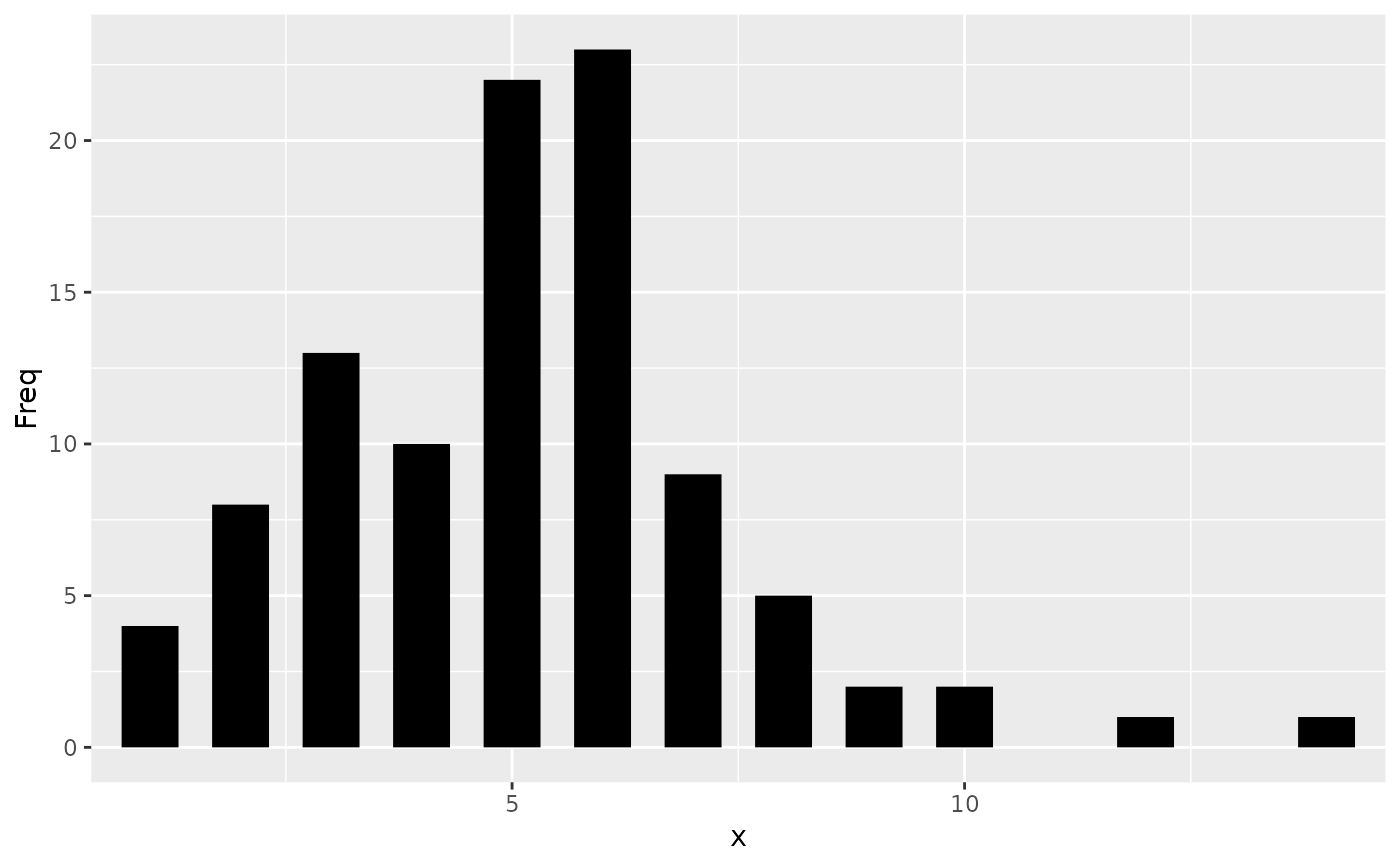
 # You can also use geom_segment() to recreate plot(type = "h")
# from base R:
counts <- as.data.frame(table(x = rpois(100, 5)))
counts$x <- as.numeric(as.character(counts$x))
with(counts, plot(x, Freq, type = "h", lwd = 10))
# You can also use geom_segment() to recreate plot(type = "h")
# from base R:
counts <- as.data.frame(table(x = rpois(100, 5)))
counts$x <- as.numeric(as.character(counts$x))
with(counts, plot(x, Freq, type = "h", lwd = 10))
 ggplot(counts, aes(x = x, y = Freq)) +
geom_segment(aes(yend = 0, xend = x), size = 10)
ggplot(counts, aes(x = x, y = Freq)) +
geom_segment(aes(yend = 0, xend = x), size = 10)