Smoothed density estimates

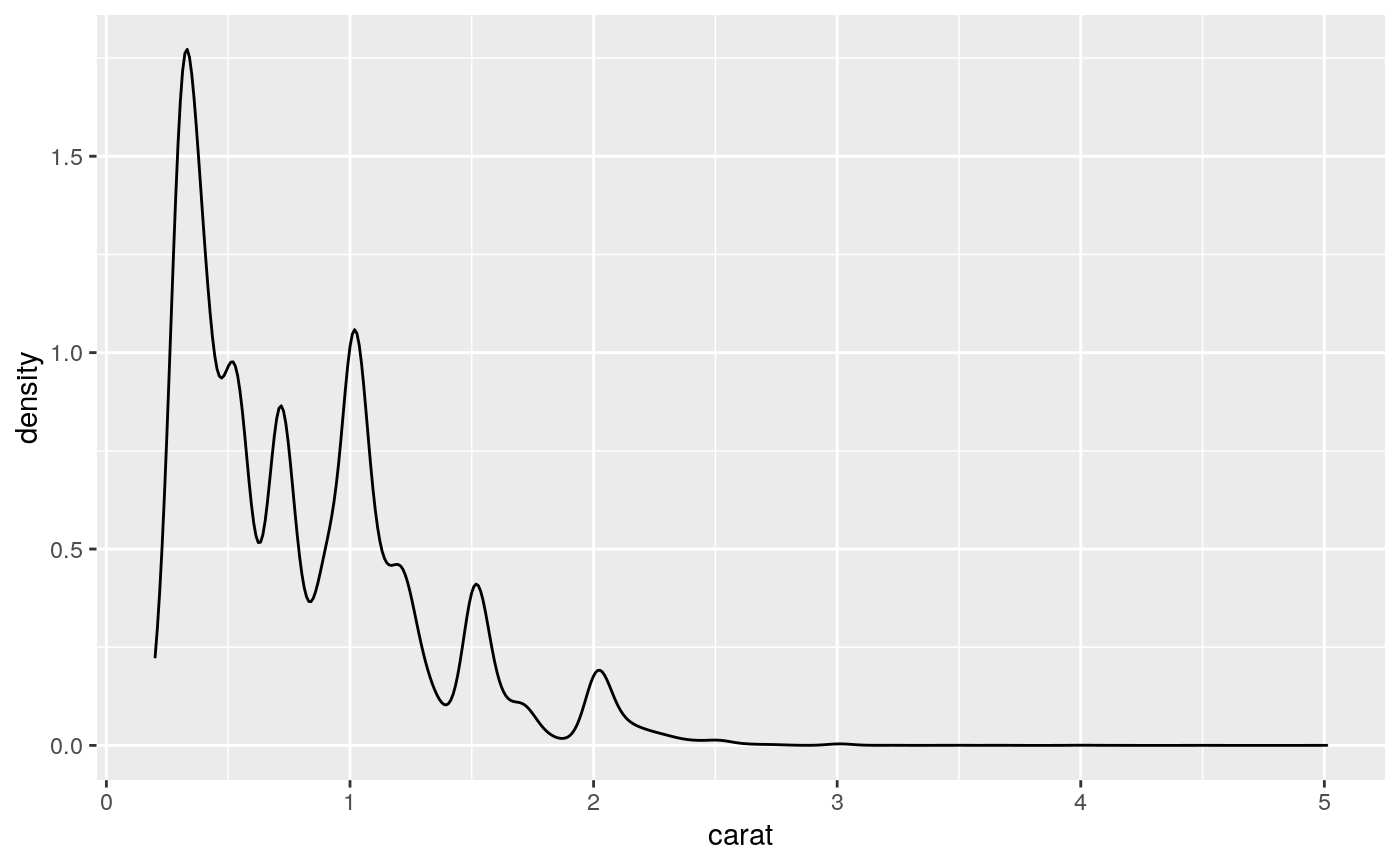
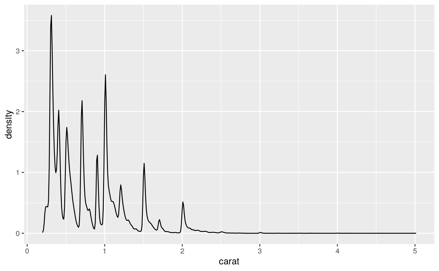
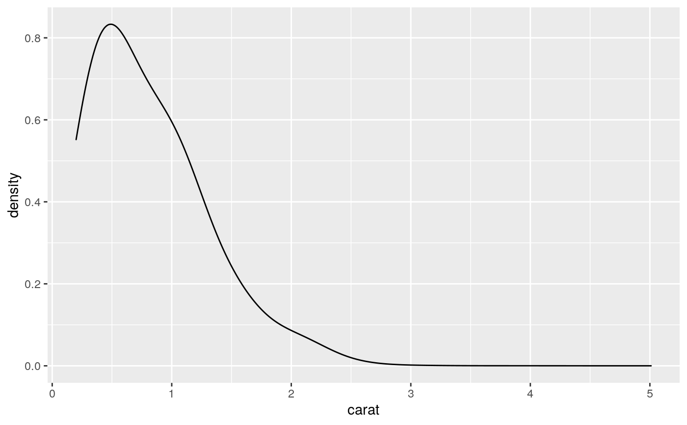
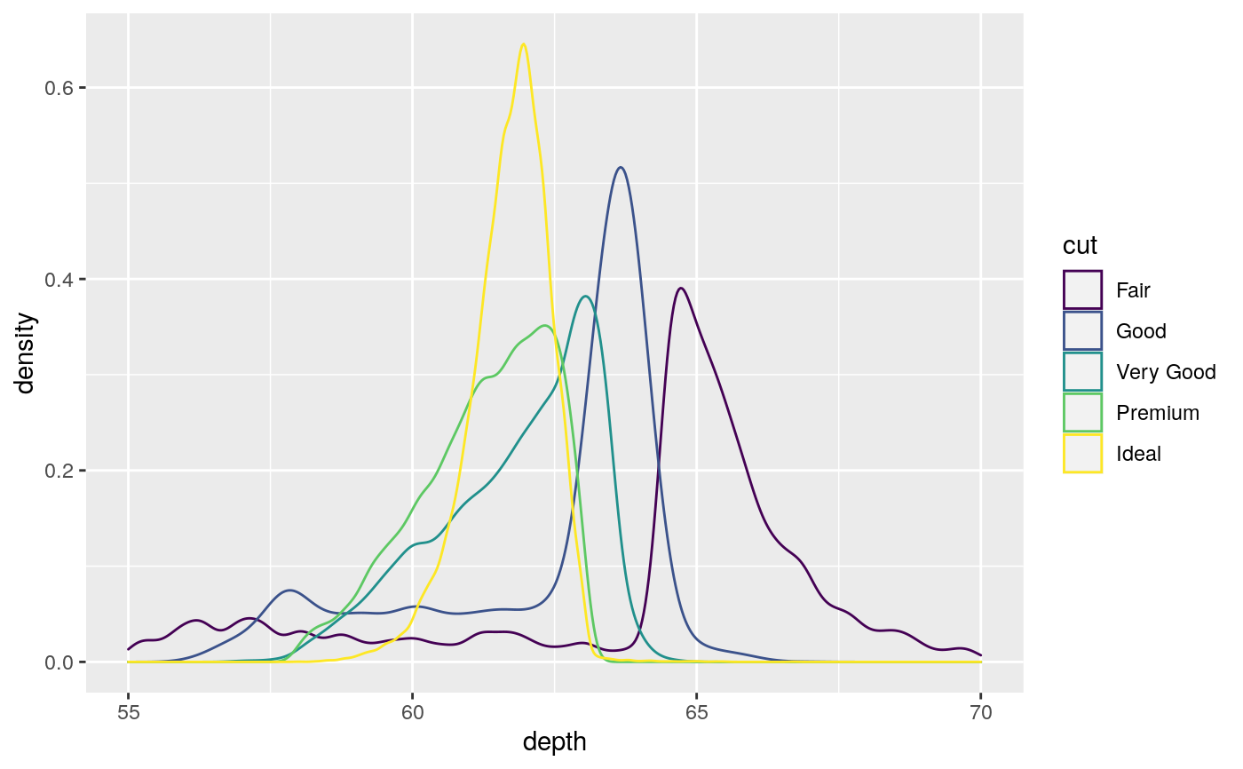
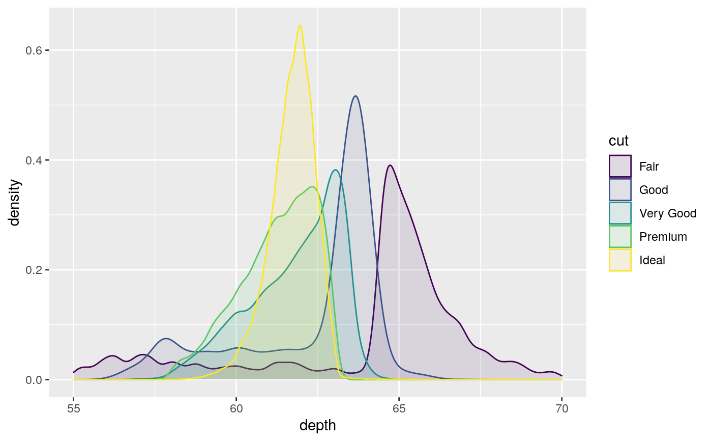
Computes and draws kernel density estimate, which is a smoothed version of the histogram. This is a useful alternative to the histogram for continuous data that comes from an underlying smooth distribution.

geom_density(
  mapping = NULL,
  data = NULL,
  stat = "density",
  position = "identity",
  ...,
  na.rm = FALSE,
  orientation = NA,
  show.legend = NA,
  inherit.aes = TRUE,
  outline.type = "upper"
)

stat_density(
  mapping = NULL,
  data = NULL,
  geom = "area",
  position = "stack",
  ...,
  bw = "nrd0",
  adjust = 1,
  kernel = "gaussian",
  n = 512,
  trim = FALSE,
  na.rm = FALSE,
  orientation = NA,
  show.legend = NA,
  inherit.aes = TRUE
)

Arguments

mapping	Set of aesthetic mappings created by aes() or aes_(). If specified and inherit.aes = TRUE (the default), it is combined with the default mapping at the top level of the plot. You must supply mapping if there is no plot mapping.
data	The data to be displayed in this layer. There are three options: If NULL, the default, the data is inherited from the plot data as specified in the call to ggplot(). A data.frame, or other object, will override the plot data. All objects will be fortified to produce a data frame. See fortify() for which variables will be created. A function will be called with a single argument, the plot data. The return value must be a data.frame, and will be used as the layer data. A function can be created from a formula (e.g. ~ head(.x, 10)).
position	Position adjustment, either as a string, or the result of a call to a position adjustment function.
...	Other arguments passed on to layer(). These are often aesthetics, used to set an aesthetic to a fixed value, like colour = "red" or size = 3. They may also be parameters to the paired geom/stat.
na.rm	If FALSE, the default, missing values are removed with a warning. If TRUE, missing values are silently removed.
orientation	The orientation of the layer. The default (NA) automatically determines the orientation from the aesthetic mapping. In the rare event that this fails it can be given explicitly by setting orientation to either "x" or "y". See the Orientation section for more detail.
show.legend	logical. Should this layer be included in the legends? NA, the default, includes if any aesthetics are mapped. FALSE never includes, and TRUE always includes. It can also be a named logical vector to finely select the aesthetics to display.
inherit.aes	If FALSE, overrides the default aesthetics, rather than combining with them. This is most useful for helper functions that define both data and aesthetics and shouldn't inherit behaviour from the default plot specification, e.g. borders().
outline.type	Type of the outline of the area; "both" draws both the upper and lower lines, "upper"/"lower" draws the either lines only. "full" draws a closed polygon around the area.
geom, stat	Use to override the default connection between geom_density and stat_density.
bw	The smoothing bandwidth to be used. If numeric, the standard deviation of the smoothing kernel. If character, a rule to choose the bandwidth, as listed in stats::bw.nrd().
adjust	A multiplicate bandwidth adjustment. This makes it possible to adjust the bandwidth while still using the a bandwidth estimator. For example, adjust = 1/2 means use half of the default bandwidth.
kernel	Kernel. See list of available kernels in density().
n	number of equally spaced points at which the density is to be estimated, should be a power of two, see density() for details
trim	This parameter only matters if you are displaying multiple densities in one plot. If FALSE, the default, each density is computed on the full range of the data. If TRUE, each density is computed over the range of that group: this typically means the estimated x values will not line-up, and hence you won't be able to stack density values.

Orientation

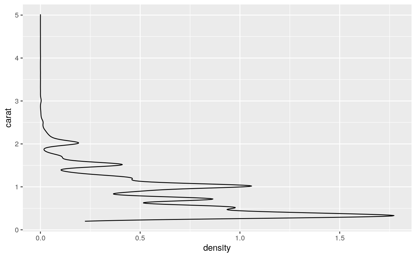
This geom treats each axis differently and, thus, can thus have two orientations. Often the orientation is easy to deduce from a combination of the given mappings and the types of positional scales in use. Thus, ggplot2 will by default try to guess which orientation the layer should have. Under rare circumstances, the orientation is ambiguous and guessing may fail. In that case the orientation can be specified directly using the orientation parameter, which can be either "x" or "y". The value gives the axis that the geom should run along, "x" being the default orientation you would expect for the geom.

Aesthetics

geom_density() understands the following aesthetics (required aesthetics are in bold):

• x

• y

• alpha

• colour

• fill

• group

• linetype

• size

• weight

Learn more about setting these aesthetics in vignette("ggplot2-specs").

Computed variables

density

density estimate

count

density * number of points - useful for stacked density plots

scaled

density estimate, scaled to maximum of 1

ndensity

alias for scaled, to mirror the syntax of stat_bin()

See also

See geom_histogram(), geom_freqpoly() for other methods of displaying continuous distribution. See geom_violin() for a compact density display.

Examples

ggplot(diamonds, aes(carat)) +
  geom_density()
# Map the values to y to flip the orientation
ggplot(diamonds, aes(y = carat)) +
  geom_density()

ggplot(diamonds, aes(carat)) +
  geom_density(adjust = 1/5)
ggplot(diamonds, aes(carat)) +
  geom_density(adjust = 5)

ggplot(diamonds, aes(depth, colour = cut)) +
  geom_density() +
  xlim(55, 70)
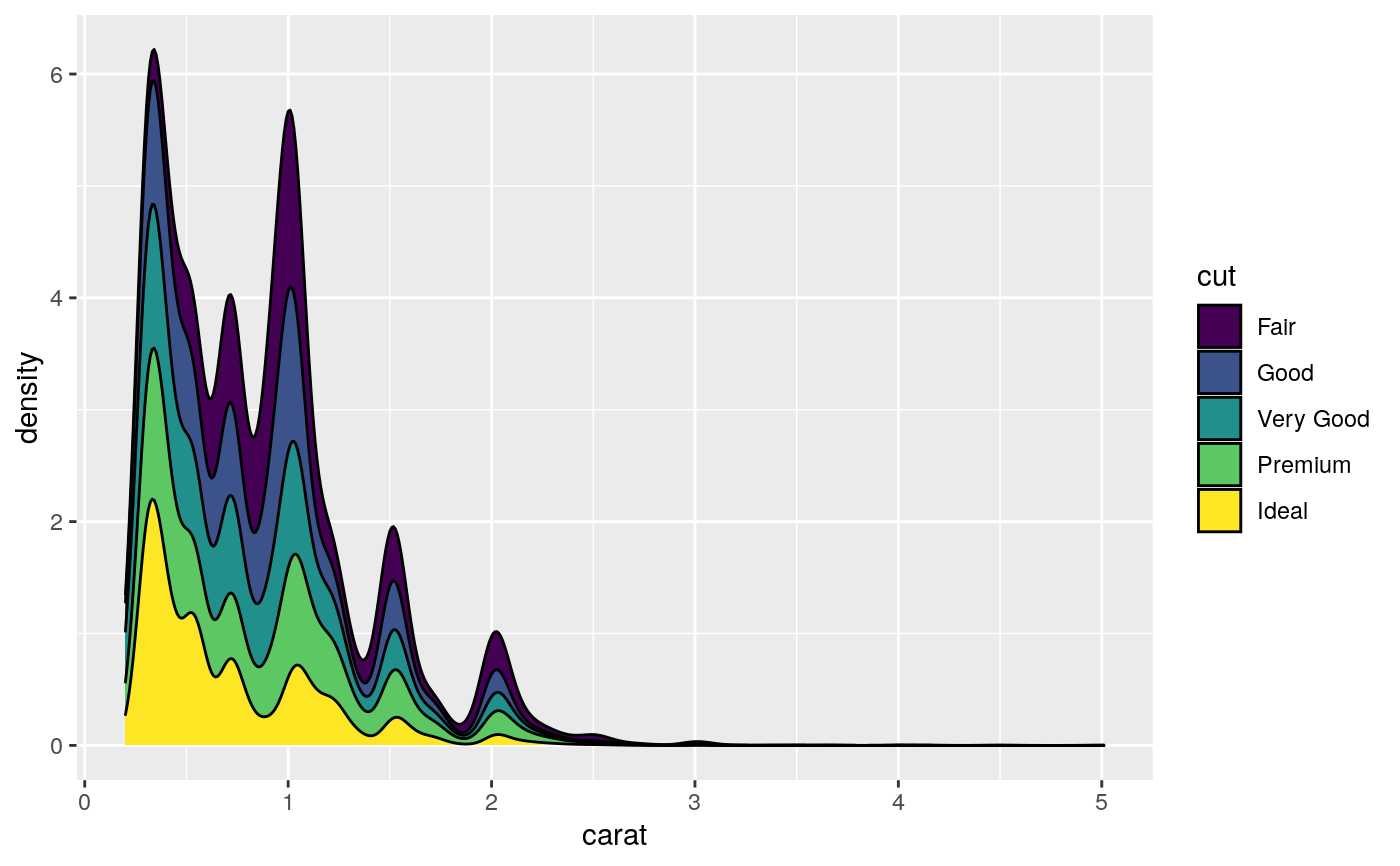
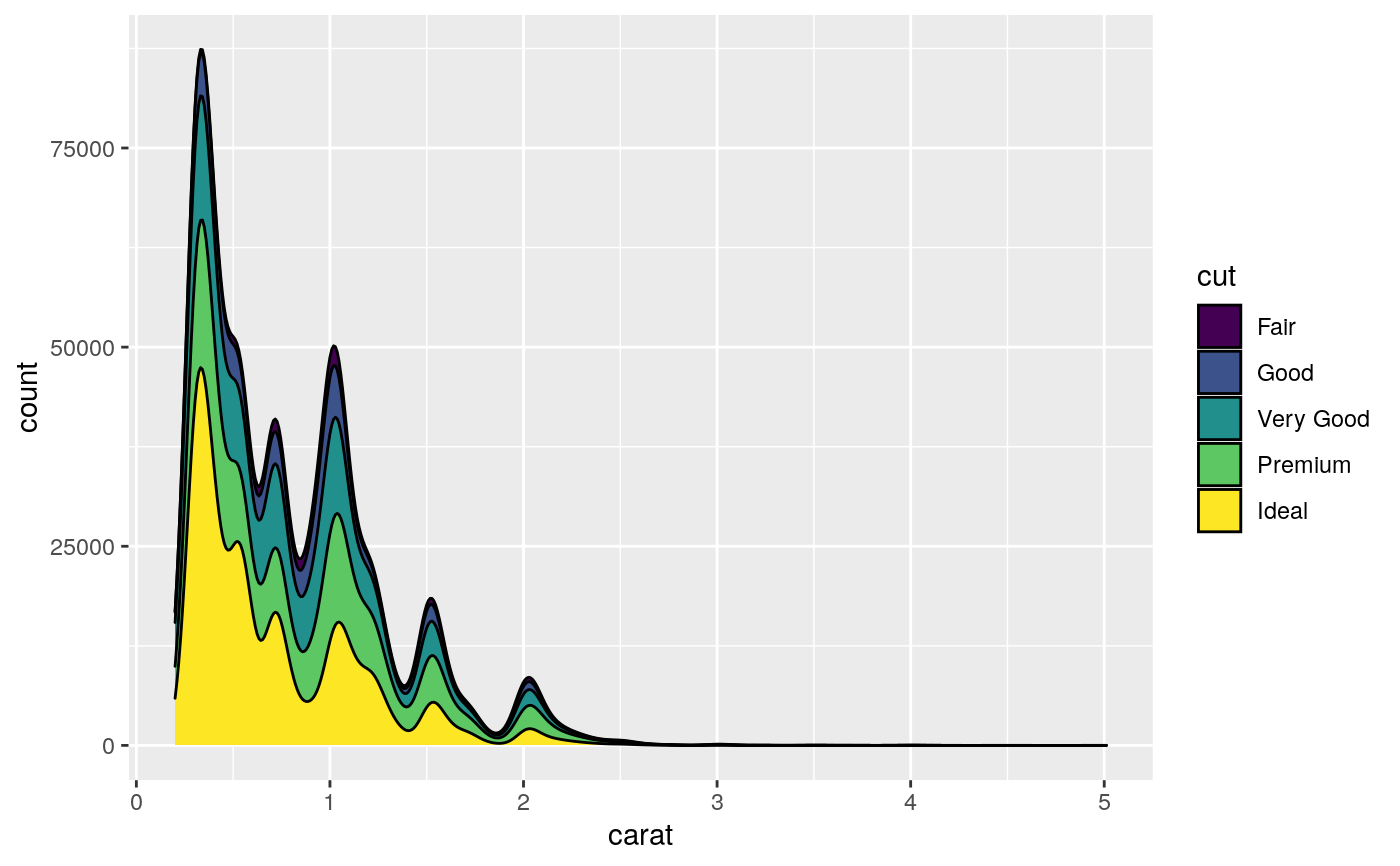
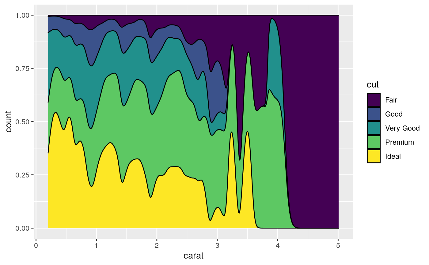
#> Warning: Removed 45 rows containing non-finite values (stat_density).
ggplot(diamonds, aes(depth, fill = cut, colour = cut)) +
  geom_density(alpha = 0.1) +
  xlim(55, 70)
#> Warning: Removed 45 rows containing non-finite values (stat_density).

# \donttest{
# Stacked density plots: if you want to create a stacked density plot, you
# probably want to 'count' (density * n) variable instead of the default
# density

# Loses marginal densities
ggplot(diamonds, aes(carat, fill = cut)) +
  geom_density(position = "stack")
# Preserves marginal densities
ggplot(diamonds, aes(carat, after_stat(count), fill = cut)) +
  geom_density(position = "stack")

# You can use position="fill" to produce a conditional density estimate
ggplot(diamonds, aes(carat, after_stat(count), fill = cut)) +
  geom_density(position = "fill")
# }