Line segments and curves

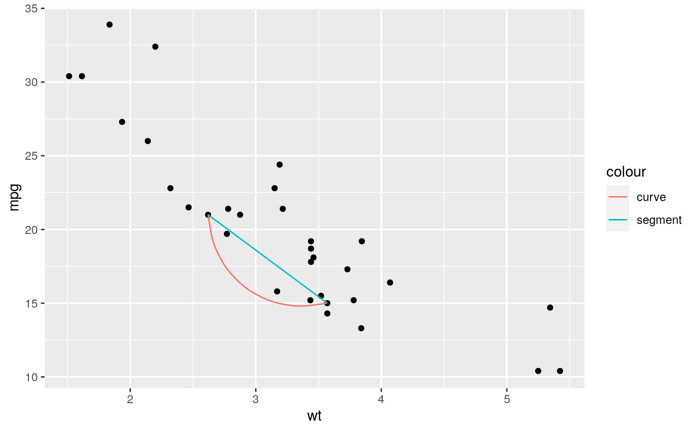
geom_segment() draws a straight line between points (x, y) and (xend, yend). geom_curve draws a curved line. See the underlying drawing function grid::curveGrob() for the parameters that control the curve.

geom_segment(
  mapping = NULL,
  data = NULL,
  stat = "identity",
  position = "identity",
  ...,
  arrow = NULL,
  arrow.fill = NULL,
  lineend = "butt",
  linejoin = "round",
  na.rm = FALSE,
  show.legend = NA,
  inherit.aes = TRUE
)

geom_curve(
  mapping = NULL,
  data = NULL,
  stat = "identity",
  position = "identity",
  ...,
  curvature = 0.5,
  angle = 90,
  ncp = 5,
  arrow = NULL,
  arrow.fill = NULL,
  lineend = "butt",
  na.rm = FALSE,
  show.legend = NA,
  inherit.aes = TRUE
)

Arguments

mapping	Set of aesthetic mappings created by `aes()` or `aes_()`. If specified and `inherit.aes = TRUE` (the default), it is combined with the default mapping at the top level of the plot. You must supply `mapping` if there is no plot mapping.
data	The data to be displayed in this layer. There are three options: If `NULL`, the default, the data is inherited from the plot data as specified in the call to `ggplot()`. A `data.frame`, or other object, will override the plot data. All objects will be fortified to produce a data frame. See `fortify()` for which variables will be created. A `function` will be called with a single argument, the plot data. The return value must be a `data.frame`, and will be used as the layer data. A `function` can be created from a `formula` (e.g. `~ head(.x, 10)`).
stat	The statistical transformation to use on the data for this layer, as a string.
position	Position adjustment, either as a string, or the result of a call to a position adjustment function.
...	Other arguments passed on to `layer()`. These are often aesthetics, used to set an aesthetic to a fixed value, like `colour = "red"` or `size = 3`. They may also be parameters to the paired geom/stat.
arrow	specification for arrow heads, as created by arrow().
arrow.fill	fill colour to use for the arrow head (if closed). `NULL` means use `colour` aesthetic.
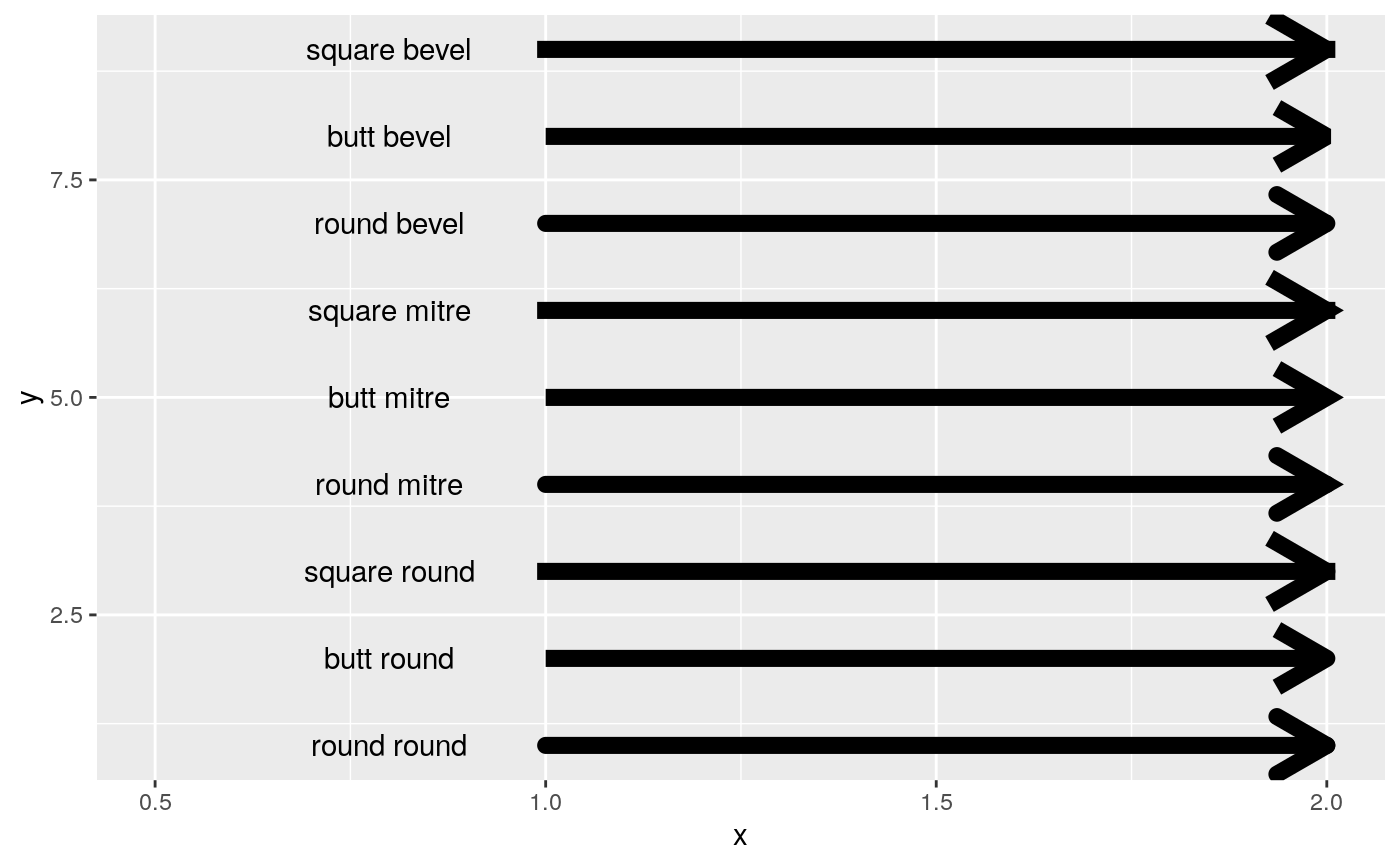
lineend	Line end style (round, butt, square).
linejoin	Line join style (round, mitre, bevel).
na.rm	If `FALSE`, the default, missing values are removed with a warning. If `TRUE`, missing values are silently removed.
show.legend	logical. Should this layer be included in the legends? `NA`, the default, includes if any aesthetics are mapped. `FALSE` never includes, and `TRUE` always includes. It can also be a named logical vector to finely select the aesthetics to display.
inherit.aes	If `FALSE`, overrides the default aesthetics, rather than combining with them. This is most useful for helper functions that define both data and aesthetics and shouldn't inherit behaviour from the default plot specification, e.g. `borders()`.
curvature	A numeric value giving the amount of curvature. Negative values produce left-hand curves, positive values produce right-hand curves, and zero produces a straight line.
angle	A numeric value between 0 and 180, giving an amount to skew the control points of the curve. Values less than 90 skew the curve towards the start point and values greater than 90 skew the curve towards the end point.
ncp	The number of control points used to draw the curve. More control points creates a smoother curve.

Details

Both geoms draw a single segment/curve per case. See geom_path if you need to connect points across multiple cases.

Aesthetics

geom_segment() understands the following aesthetics (required aesthetics are in bold):

x
y
xend
yend
alpha
colour
group
linetype
size

Learn more about setting these aesthetics in vignette("ggplot2-specs").

Examples

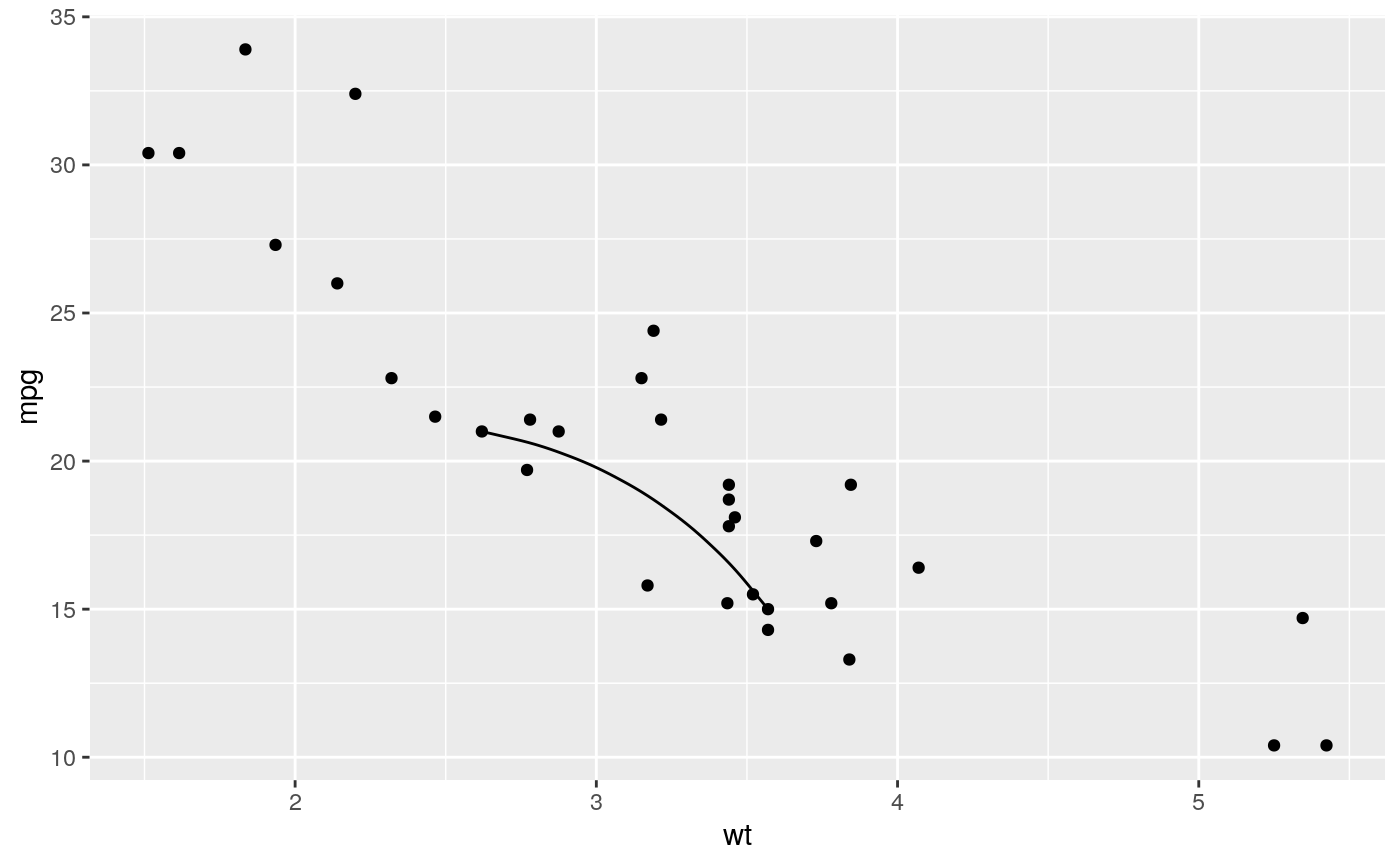
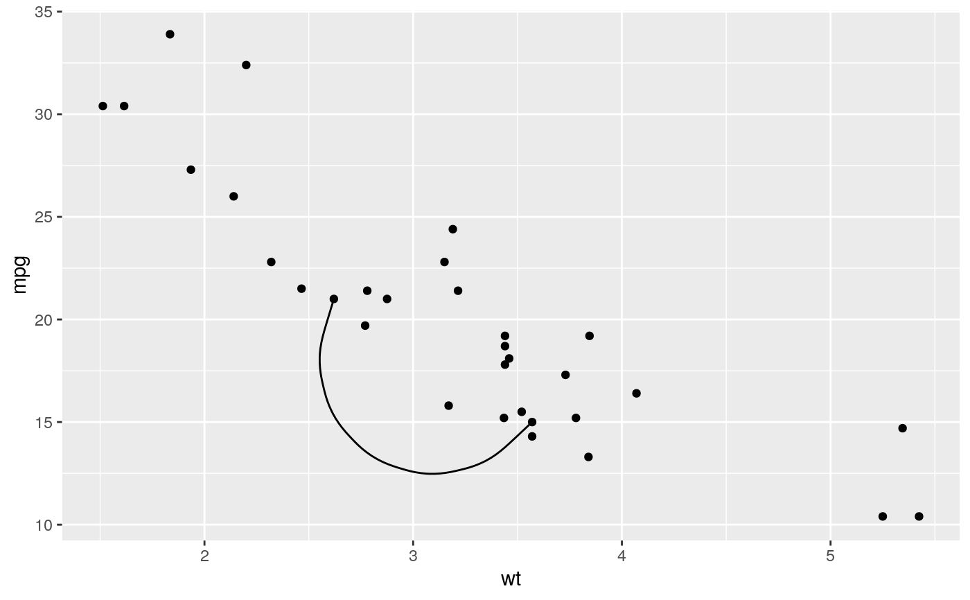
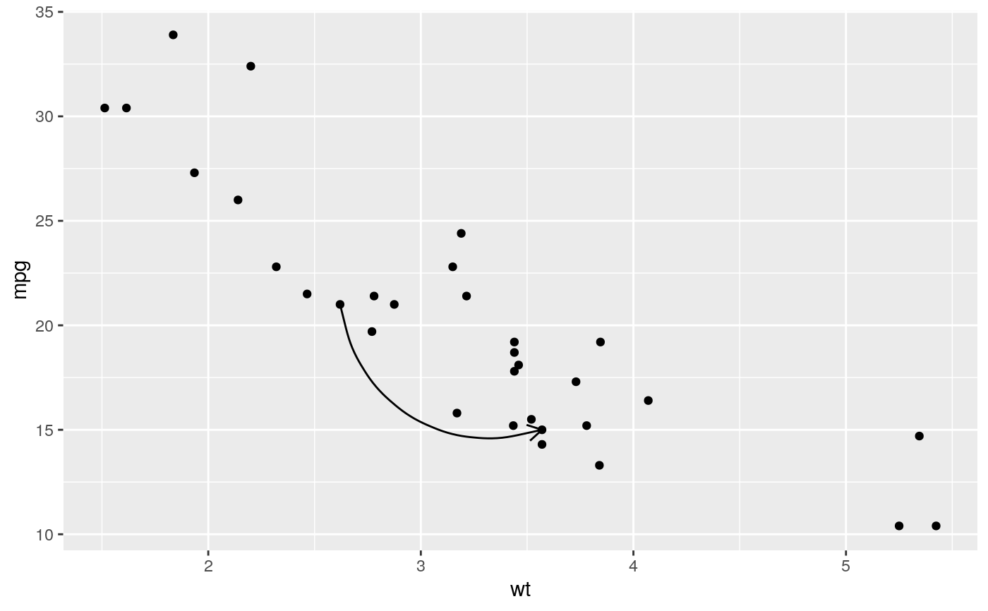
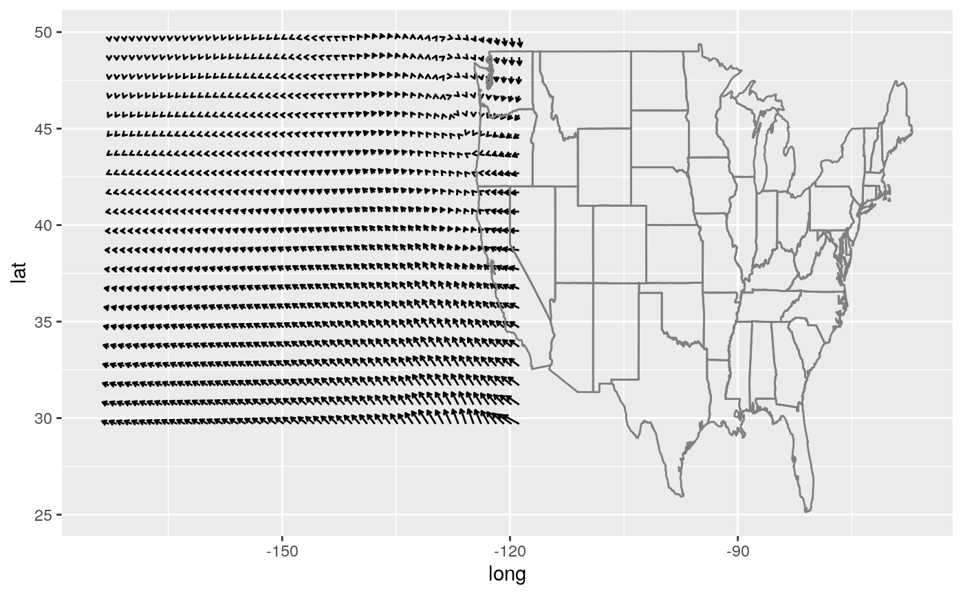
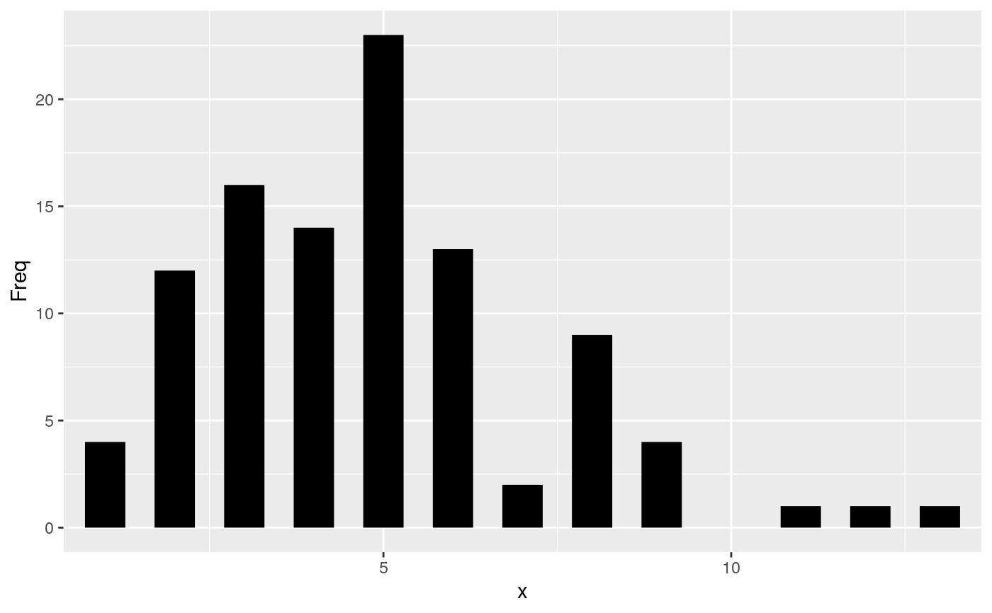
b <- ggplot(mtcars, aes(wt, mpg)) +
  geom_point()

df <- data.frame(x1 = 2.62, x2 = 3.57, y1 = 21.0, y2 = 15.0)
b +
 geom_curve(aes(x = x1, y = y1, xend = x2, yend = y2, colour = "curve"), data = df) +
 geom_segment(aes(x = x1, y = y1, xend = x2, yend = y2, colour = "segment"), data = df)

b + geom_curve(aes(x = x1, y = y1, xend = x2, yend = y2), data = df, curvature = -0.2)
b + geom_curve(aes(x = x1, y = y1, xend = x2, yend = y2), data = df, curvature = 1)
b + geom_curve(
  aes(x = x1, y = y1, xend = x2, yend = y2),
  data = df,
  arrow = arrow(length = unit(0.03, "npc"))
)

ggplot(seals, aes(long, lat)) +
  geom_segment(aes(xend = long + delta_long, yend = lat + delta_lat),
    arrow = arrow(length = unit(0.1,"cm"))) +
  borders("state")

# Use lineend and linejoin to change the style of the segments
df2 <- expand.grid(
  lineend = c('round', 'butt', 'square'),
  linejoin = c('round', 'mitre', 'bevel'),
  stringsAsFactors = FALSE
)
df2 <- data.frame(df2, y = 1:9)
ggplot(df2, aes(x = 1, y = y, xend = 2, yend = y, label = paste(lineend, linejoin))) +
  geom_segment(
     lineend = df2$lineend, linejoin = df2$linejoin,
     size = 3, arrow = arrow(length = unit(0.3, "inches"))
  ) +
  geom_text(hjust = 'outside', nudge_x = -0.2) +
  xlim(0.5, 2)

# You can also use geom_segment to recreate plot(type = "h") :
counts <- as.data.frame(table(x = rpois(100,5)))
counts$x <- as.numeric(as.character(counts$x))
with(counts, plot(x, Freq, type = "h", lwd = 10))

ggplot(counts, aes(x, Freq)) +
  geom_segment(aes(xend = x, yend = 0), size = 10, lineend = "butt")

Arguments

Details

Aesthetics

See also

Examples