Summarise y values at unique/binned x

stat_summary() operates on unique x or y; stat_summary_bin() operates on binned x or y. They are more flexible versions of stat_bin(): instead of just counting, they can compute any aggregate.

stat_summary_bin(
  mapping = NULL,
  data = NULL,
  geom = "pointrange",
  position = "identity",
  ...,
  fun.data = NULL,
  fun = NULL,
  fun.max = NULL,
  fun.min = NULL,
  fun.args = list(),
  bins = 30,
  binwidth = NULL,
  breaks = NULL,
  na.rm = FALSE,
  orientation = NA,
  show.legend = NA,
  inherit.aes = TRUE,
  fun.y,
  fun.ymin,
  fun.ymax
)

stat_summary(
  mapping = NULL,
  data = NULL,
  geom = "pointrange",
  position = "identity",
  ...,
  fun.data = NULL,
  fun = NULL,
  fun.max = NULL,
  fun.min = NULL,
  fun.args = list(),
  na.rm = FALSE,
  orientation = NA,
  show.legend = NA,
  inherit.aes = TRUE,
  fun.y,
  fun.ymin,
  fun.ymax
)

Arguments

mapping	Set of aesthetic mappings created by `aes()` or `aes_()`. If specified and `inherit.aes = TRUE` (the default), it is combined with the default mapping at the top level of the plot. You must supply `mapping` if there is no plot mapping.
data	The data to be displayed in this layer. There are three options: If `NULL`, the default, the data is inherited from the plot data as specified in the call to `ggplot()`. A `data.frame`, or other object, will override the plot data. All objects will be fortified to produce a data frame. See `fortify()` for which variables will be created. A `function` will be called with a single argument, the plot data. The return value must be a `data.frame`, and will be used as the layer data. A `function` can be created from a `formula` (e.g. `~ head(.x, 10)`).
geom	Use to override the default connection between `geom_histogram()`/`geom_freqpoly()` and `stat_bin()`.
position	Position adjustment, either as a string, or the result of a call to a position adjustment function.
...	Other arguments passed on to `layer()`. These are often aesthetics, used to set an aesthetic to a fixed value, like `colour = "red"` or `size = 3`. They may also be parameters to the paired geom/stat.
fun.data	A function that is given the complete data and should return a data frame with variables `ymin`, `y`, and `ymax`.
fun.min, fun, fun.max	Alternatively, supply three individual functions that are each passed a vector of values and should return a single number.
fun.args	Optional additional arguments passed on to the functions.
bins	Number of bins. Overridden by `binwidth`. Defaults to 30.
binwidth	The width of the bins. Can be specified as a numeric value or as a function that calculates width from unscaled x. Here, "unscaled x" refers to the original x values in the data, before application of any scale transformation. When specifying a function along with a grouping structure, the function will be called once per group. The default is to use the number of bins in `bins`, covering the range of the data. You should always override this value, exploring multiple widths to find the best to illustrate the stories in your data. The bin width of a date variable is the number of days in each time; the bin width of a time variable is the number of seconds.
breaks	Alternatively, you can supply a numeric vector giving the bin boundaries. Overrides `binwidth`, `bins`, `center`, and `boundary`.
na.rm	If `FALSE`, the default, missing values are removed with a warning. If `TRUE`, missing values are silently removed.
orientation	The orientation of the layer. The default (`NA`) automatically determines the orientation from the aesthetic mapping. In the rare event that this fails it can be given explicitly by setting `orientation` to either `"x"` or `"y"`. See the Orientation section for more detail.
show.legend	logical. Should this layer be included in the legends? `NA`, the default, includes if any aesthetics are mapped. `FALSE` never includes, and `TRUE` always includes. It can also be a named logical vector to finely select the aesthetics to display.
inherit.aes	If `FALSE`, overrides the default aesthetics, rather than combining with them. This is most useful for helper functions that define both data and aesthetics and shouldn't inherit behaviour from the default plot specification, e.g. `borders()`.
fun.ymin, fun.y, fun.ymax	Deprecated, use the versions specified above instead.

Orientation

This geom treats each axis differently and, thus, can thus have two orientations. Often the orientation is easy to deduce from a combination of the given mappings and the types of positional scales in use. Thus, ggplot2 will by default try to guess which orientation the layer should have. Under rare circumstances, the orientation is ambiguous and guessing may fail. In that case the orientation can be specified directly using the orientation parameter, which can be either "x" or "y". The value gives the axis that the geom should run along, "x" being the default orientation you would expect for the geom.

Aesthetics

stat_summary() understands the following aesthetics (required aesthetics are in bold):

x
y
group

Learn more about setting these aesthetics in vignette("ggplot2-specs").

Summary functions

You can either supply summary functions individually (fun, fun.max, fun.min), or as a single function (fun.data):

fun.data

Complete summary function. Should take numeric vector as input and return data frame as output

fun.min

min summary function (should take numeric vector and return single number)

fun

main summary function (should take numeric vector and return single number)

fun.max

max summary function (should take numeric vector and return single number)

A simple vector function is easiest to work with as you can return a single number, but is somewhat less flexible. If your summary function computes multiple values at once (e.g. min and max), use fun.data.

fun.data will recieve data as if it was oriented along the x-axis and should return a data.frame that corresponds to that orientation. The layer will take care of flipping the input and output if it is oriented along the y-axis.

If no aggregation functions are supplied, will default to mean_se().

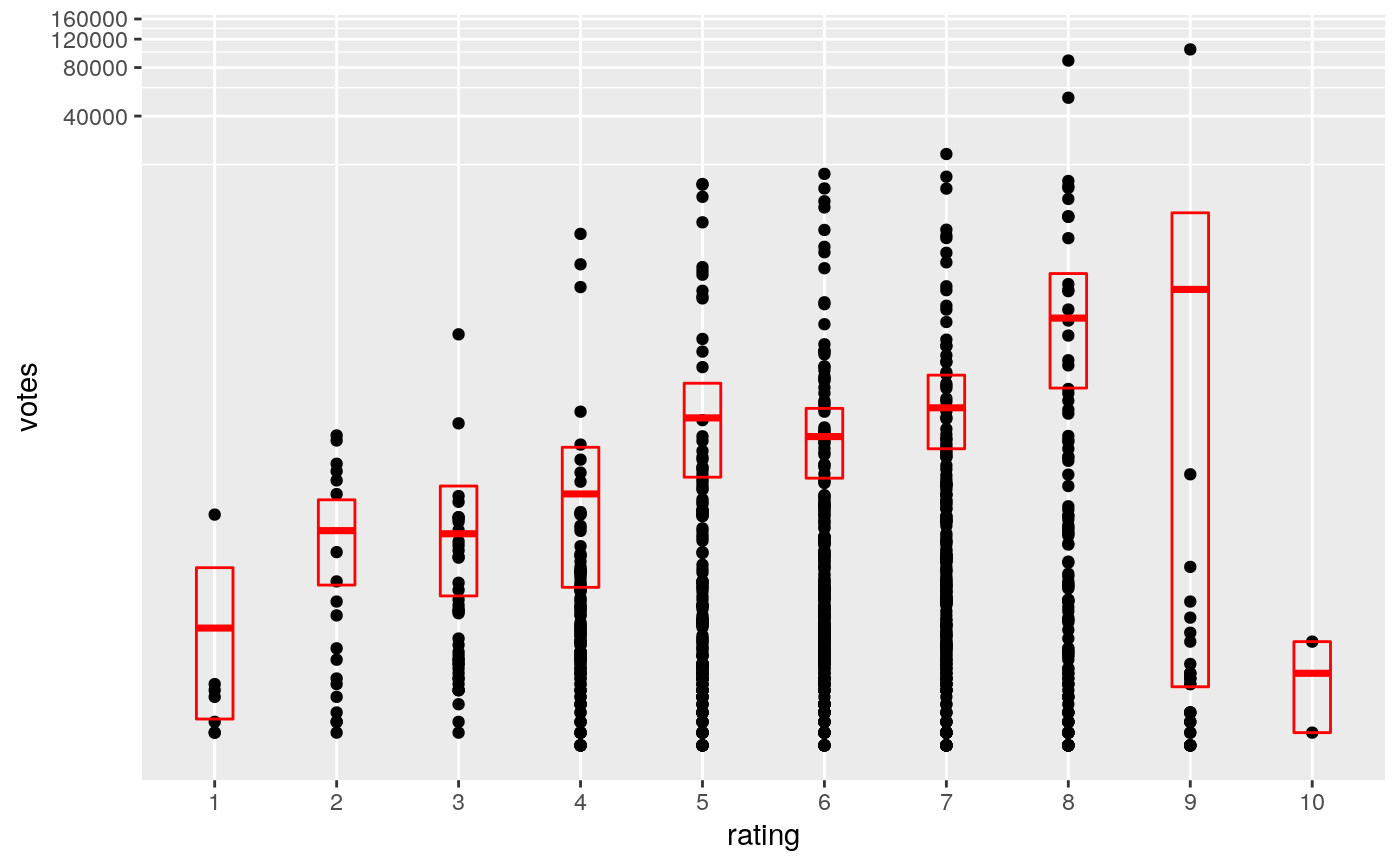
Examples

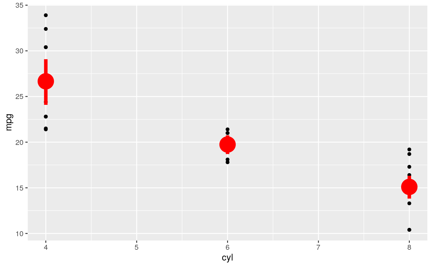
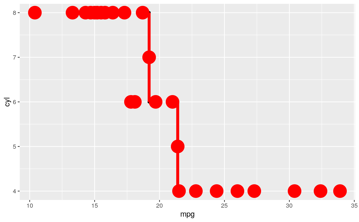
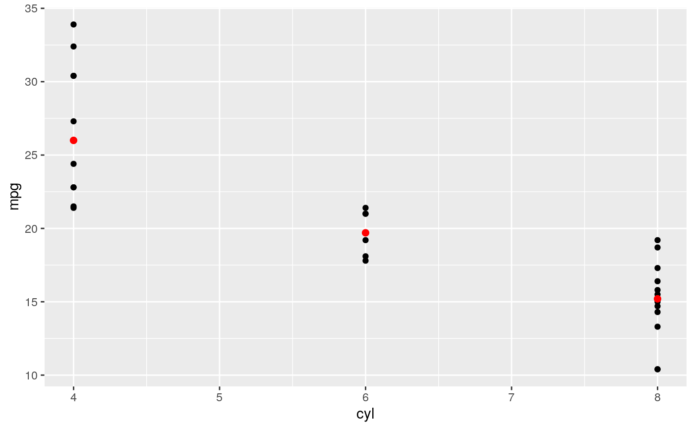
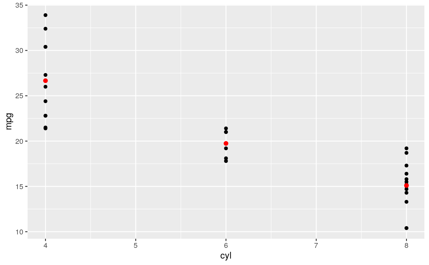
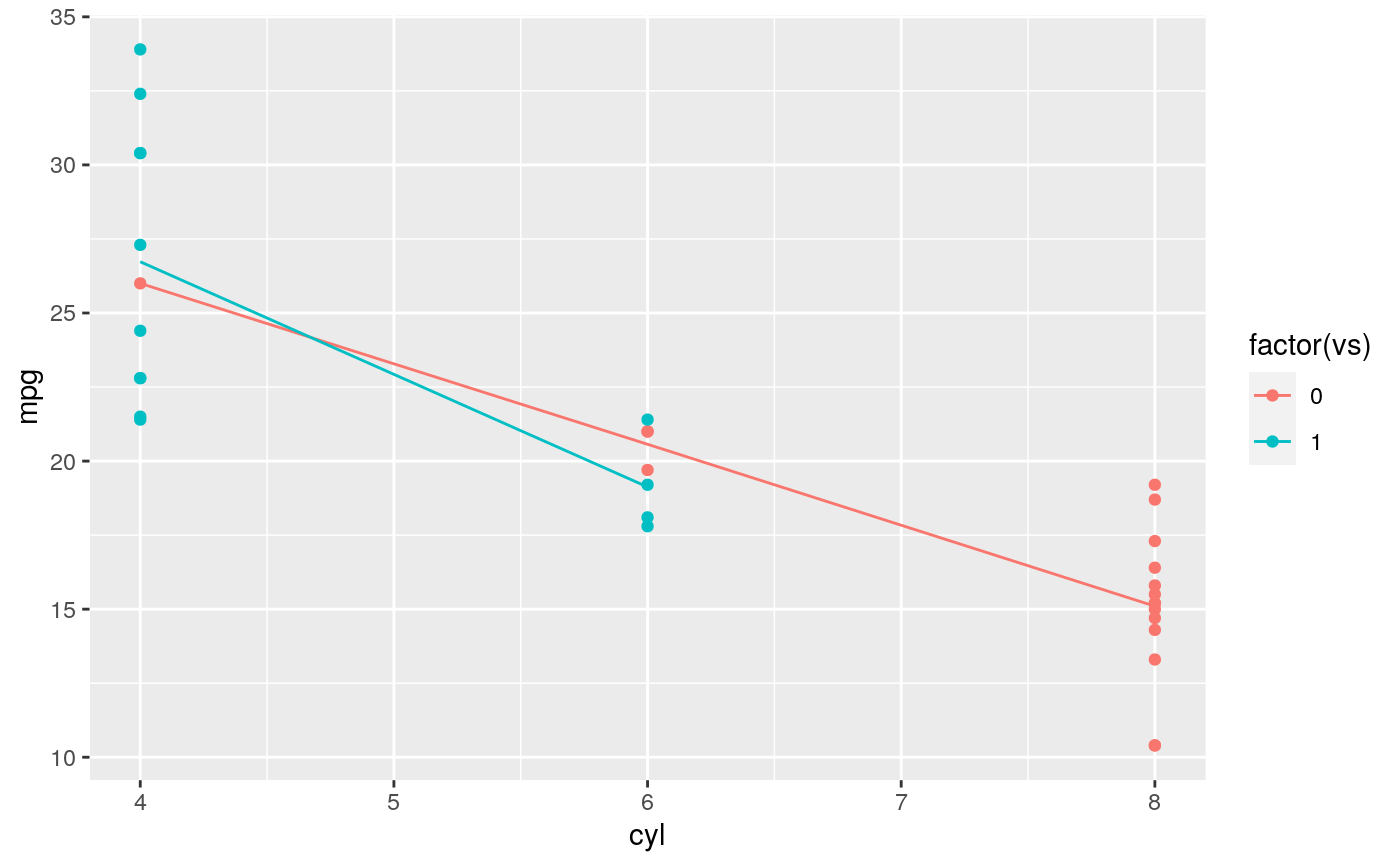
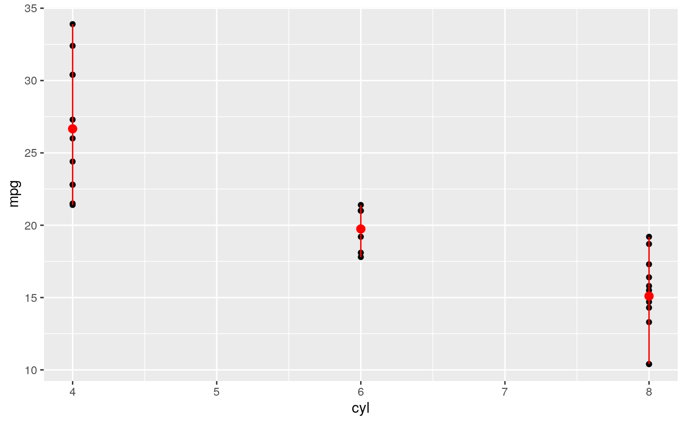
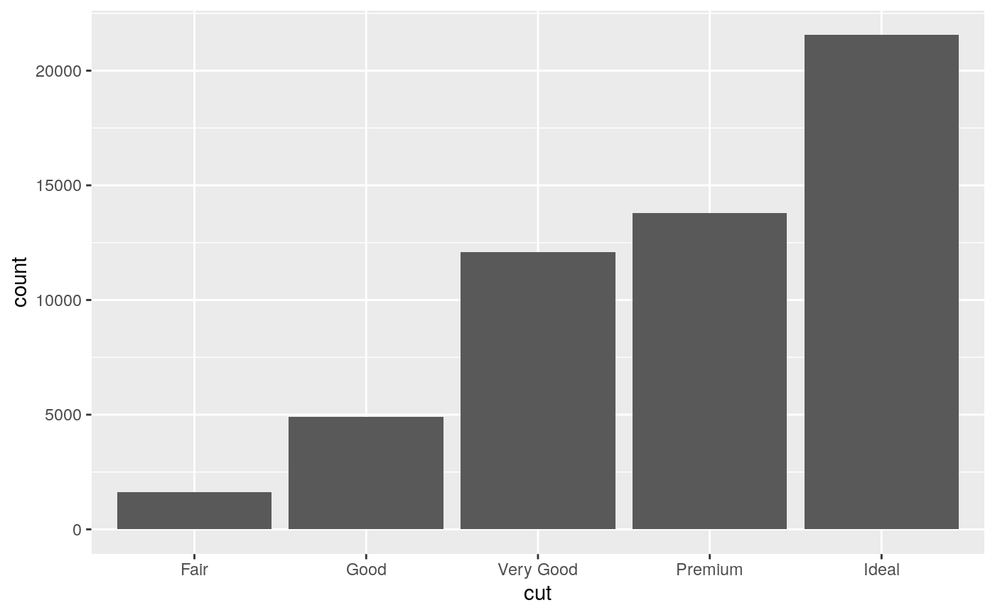
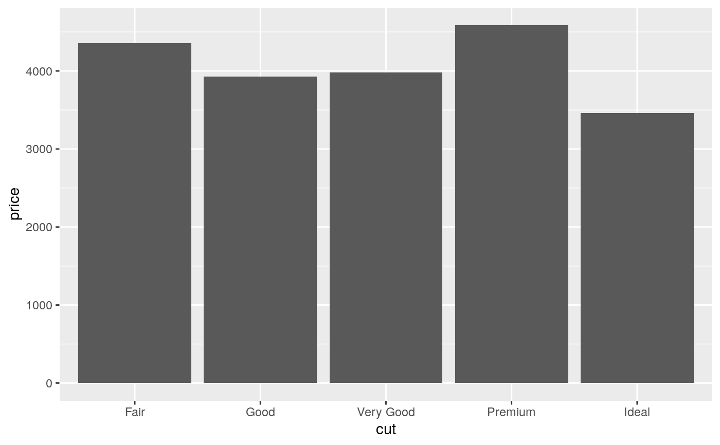
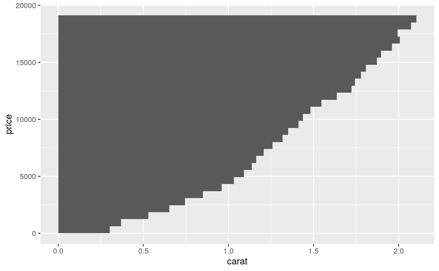
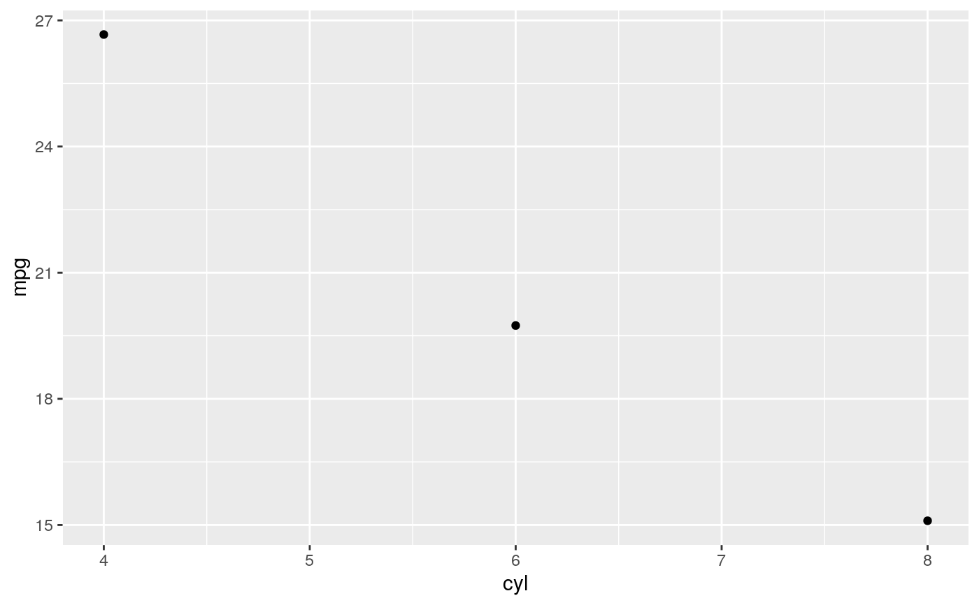
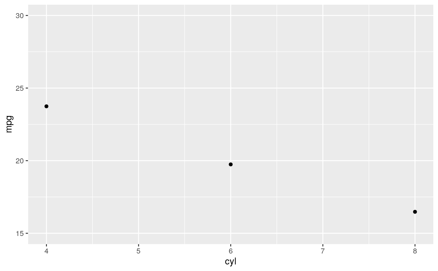
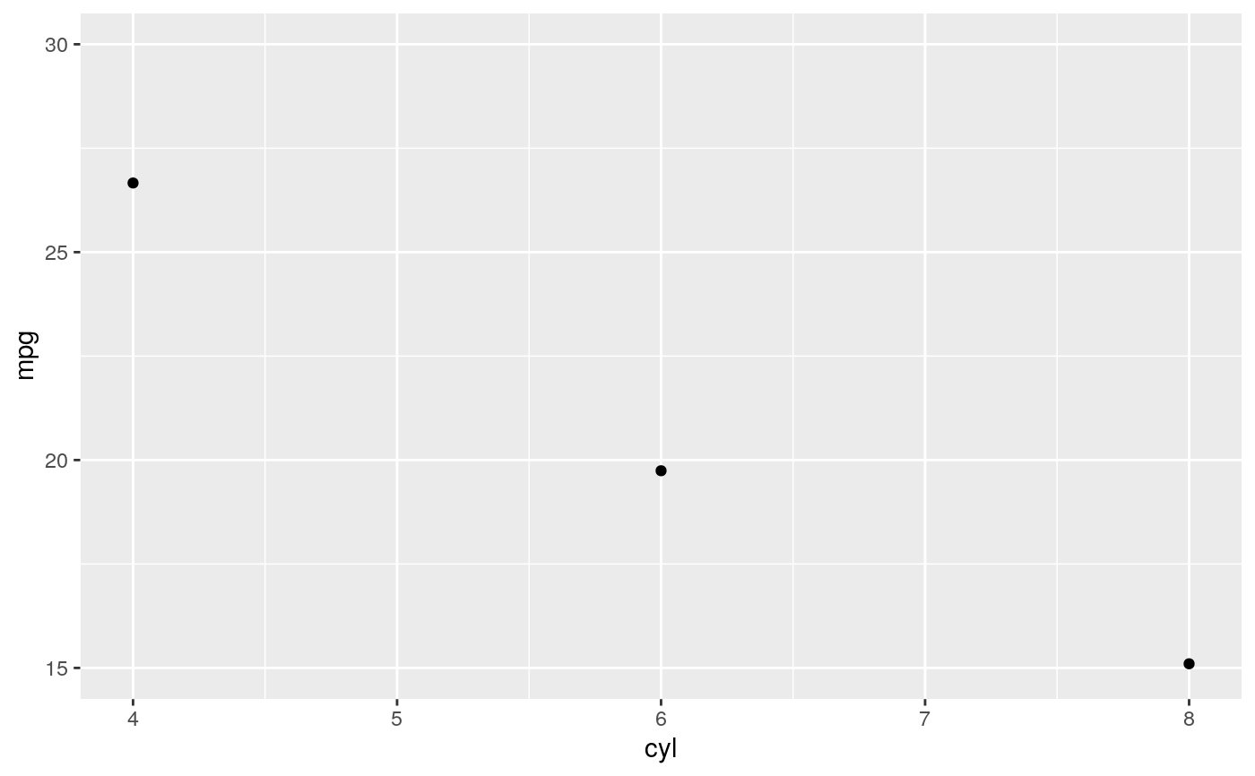
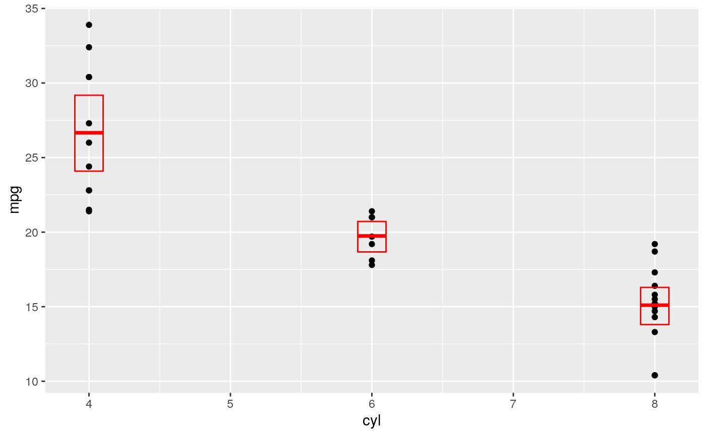
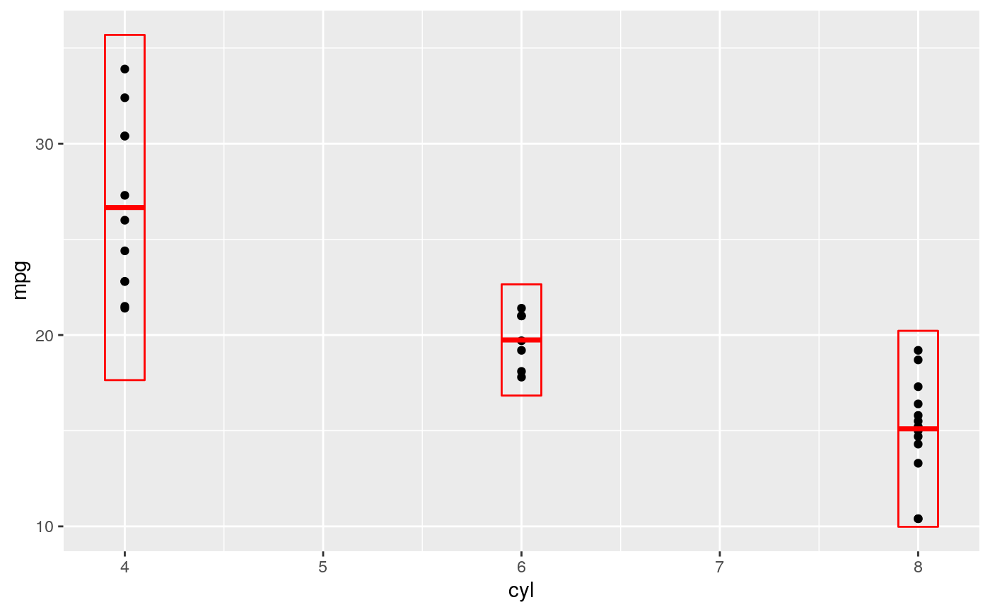
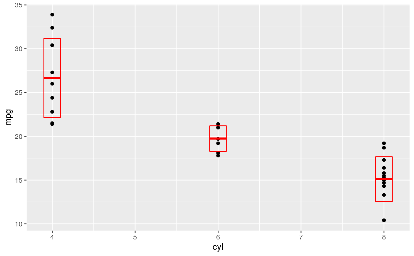
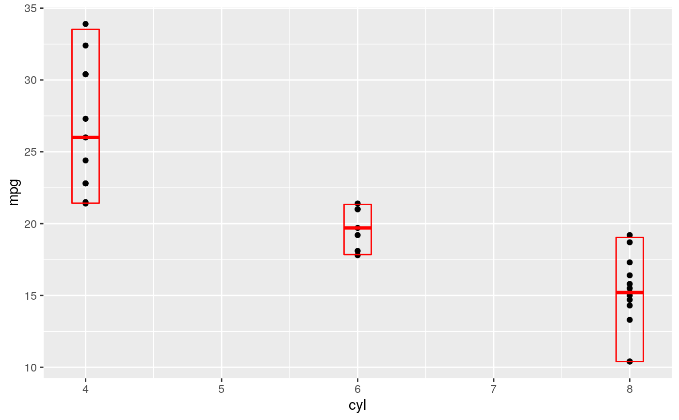
d <- ggplot(mtcars, aes(cyl, mpg)) + geom_point()
d + stat_summary(fun.data = "mean_cl_boot", colour = "red", size = 2)

# Orientation follows the discrete axis
ggplot(mtcars, aes(mpg, cyl)) +
  geom_point() +
  stat_summary(fun.data = "mean_cl_boot", colour = "red", size = 2)
#> Warning: Removed 18 rows containing missing values (geom_segment).

# You can supply individual functions to summarise the value at
# each x:
d + stat_summary(fun = "median", colour = "red", size = 2, geom = "point")
d + stat_summary(fun = "mean", colour = "red", size = 2, geom = "point")
d + aes(colour = factor(vs)) + stat_summary(fun = mean, geom="line")

d + stat_summary(fun = mean, fun.min = min, fun.max = max,
  colour = "red")

d <- ggplot(diamonds, aes(cut))
d + geom_bar()
d + stat_summary(aes(y = price), fun = "mean", geom = "bar")

# Orientation of stat_summary_bin is ambiguous and must be specified directly
ggplot(diamonds, aes(carat, price)) +
  stat_summary_bin(fun = "mean", geom = "bar", orientation = 'y')

# \donttest{
# Don't use ylim to zoom into a summary plot - this throws the
# data away
p <- ggplot(mtcars, aes(cyl, mpg)) +
  stat_summary(fun = "mean", geom = "point")
p
p + ylim(15, 30)
#> Warning: Removed 9 rows containing non-finite values (stat_summary).
# Instead use coord_cartesian
p + coord_cartesian(ylim = c(15, 30))

# A set of useful summary functions is provided from the Hmisc package:
stat_sum_df <- function(fun, geom="crossbar", ...) {
  stat_summary(fun.data = fun, colour = "red", geom = geom, width = 0.2, ...)
}
d <- ggplot(mtcars, aes(cyl, mpg)) + geom_point()
# The crossbar geom needs grouping to be specified when used with
# a continuous x axis.
d + stat_sum_df("mean_cl_boot", mapping = aes(group = cyl))
d + stat_sum_df("mean_sdl", mapping = aes(group = cyl))
d + stat_sum_df("mean_sdl", fun.args = list(mult = 1), mapping = aes(group = cyl))
d + stat_sum_df("median_hilow", mapping = aes(group = cyl))

# An example with highly skewed distributions:
if (require("ggplot2movies")) {
set.seed(596)
mov <- movies[sample(nrow(movies), 1000), ]
 m2 <- ggplot(mov, aes(x = factor(round(rating)), y = votes)) + geom_point()
 m2 <- m2 + stat_summary(fun.data = "mean_cl_boot", geom = "crossbar",
                         colour = "red", width = 0.3) + xlab("rating")
m2
# Notice how the overplotting skews off visual perception of the mean
# supplementing the raw data with summary statistics is _very_ important

# Next, we'll look at votes on a log scale.

# Transforming the scale means the data are transformed
# first, after which statistics are computed:
m2 + scale_y_log10()
# Transforming the coordinate system occurs after the
# statistic has been computed. This means we're calculating the summary on the raw data
# and stretching the geoms onto the log scale.  Compare the widths of the
# standard errors.
m2 + coord_trans(y="log10")
}
# }

Arguments

Orientation

Aesthetics

Summary functions

See also

Examples