Use yspec to document analysis data sets and utilize data attributes in a modeling and simulation workflow.
Installation
You can install the development version of yspec from GitHub with:
# install.packages("devtools")
devtools::install_github("metrumresearchgroup/yspec")
Create a yspec object
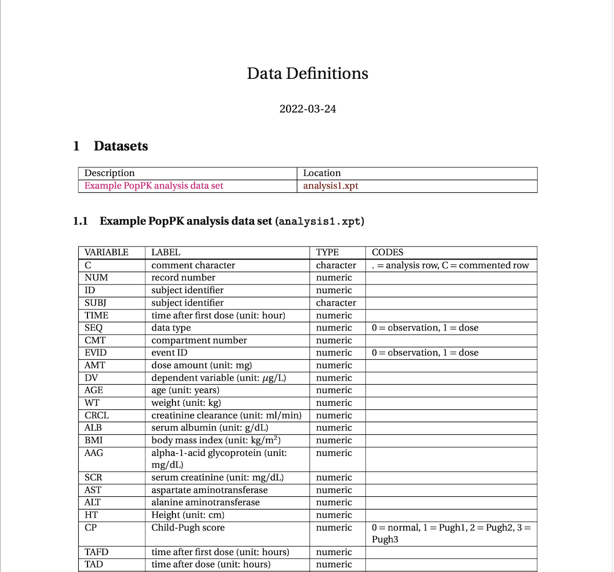
Before or while programming an analysis data set, write out data definitions in yaml format:
library(yspec)
library(dplyr)
library(tidyr)

readLines("inst/internal/analysis1.yml")[1:20] %>% writeLines()
. SETUP__:
.   description: Example PopPK analysis data set
.   sponsor: example-project
.   projectnumber: EXAMPK1011F
.   use_internal_db: true
.   glue:
.     bmiunits: "kg/m$^2$"
.   flags:
.     covariate: [AGE:SCR, HT, AST:ALT]
.   lookup_file: "look.yml"
.   extend_file: "analysis1-ext.yml"
. C:
. NUM:
. ID:
. SUBJ: !look
. TIME: !look
.   label: time after first dose
.   unit: hour
. SEQ:
.   label: data type
Now use yspec to read that into a object in R
spec <- ys_load("inst/internal/analysis1.yml")Query this object to get a sense of what is in the data overall
head(spec)
.    name info         unit              short        source
. 1     C  cd-            .  comment character ysdb_internal
. 2   NUM  ---            .      record number ysdb_internal
. 3    ID  ---            . subject identifier ysdb_internal
. 4  SUBJ  c--            . subject identifier ysdb_internal
. 5  TIME  ---         hour               TIME          look
. 6   SEQ  -d-            .                SEQ             .
. 7   CMT  ---            . compartment number ysdb_internal
. 8  EVID  -d-            .           event ID ysdb_internal
. 9   AMT  ---           mg        dose amount ysdb_internal
. 10   DV  --- micrograms/L dependent variable ysdb_internal
or on a column by column basis for continuous data
spec$WT
.  name  value
.  col   WT
.  type  numeric
.  short weight
.  unit  kg
.  range 40 to 100
as well as categorical data
spec$BLQ
.  name  value
.  col   BLQ
.  type  numeric
.  short below limit of quantification
.  value 0 : above QL
.        1 : below QL
And we can render a define.pdf file as well
Using yspec
This section illustrates a few examples for how yspec might be used (other than creating define.pdf).
To make it easier to get started with yspec, we’ve included example data and corresponding yspec object in the package
data <- ys_help$data()
spec <- ys_help$spec()
Add factors
When you have discrete data, “decodes” can be provided and used to create factors in the data. We have that for the RF column
spec$RF
.  name  value
.  col   RF
.  type  character
.  short renal function stage
.  value norm : Normal
.        mild : Mild
.        mod  : Moderate
.        sev  : Severe
Now we’ll have a column called RF_f which is a factor version of RF
ys_add_factors(data, spec, RF) %>% count(RF, RF_f)
.     RF     RF_f    n
. 1 mild     Mild  360
. 2  mod Moderate  360
. 3 norm   Normal 3280
. 4  sev   Severe  360
Recode
Every column can have a “short” name; for WT it is
spec$WT$short
. [1] "weight"
Every continuous data can also have a unit; again for WT
spec$WT$unit
. [1] "kg"
We use the spec to “recode” using this information. First create a data summary in long format
summ <-
  data %>%
  select(WT, ALB, AGE) %>%
  pivot_longer(everything()) %>%
  group_by(name) %>%
  summarise(Mean = mean(value), Sd = sd(value))

summ
. # A tibble: 3 × 3
.   name   Mean     Sd
.   <chr> <dbl>  <dbl>
. 1 AGE   33.8   8.60
. 2 ALB    4.30  0.707
. 3 WT    70.9  12.8
To recode, pull the information from spec
summ %>%
  mutate(name = ys_recode(name, spec,  unit = TRUE, title_case = TRUE))
. # A tibble: 3 × 3
.   name            Mean     Sd
.   <chr>          <dbl>  <dbl>
. 1 Age (years)    33.8   8.60
. 2 Albumin (g/dL)  4.30  0.707
. 3 Weight (kg)    70.9  12.8
Manipulating yspec
There are several functions for working on your yspec object
Select some columns
body_size <- ys_select(spec, WT, BMI, HT)

body_size
.  name info unit  short  source
.  WT   ---  kg    weight ysdb_internal
.  BMI  ---  m2/kg BMI    ysdb_internal
.  HT   ---  cm    height ysdb_internal
Filter based on some flags that were set
ys_filter(spec, covariate)
.  name info unit   short                      source
.  AGE  ---  years  age                        ysdb_internal
.  WT   ---  kg     weight                     ysdb_internal
.  CRCL ---  ml/min CRCL                       .
.  ALB  ---  g/dL   albumin                    ysdb_internal
.  BMI  ---  m2/kg  BMI                        ysdb_internal
.  AAG  ---  mg/dL  alpha-1-acid glycoprotein  .
.  SCR  ---  mg/dL  serum creatinine           .
.  AST  ---  .      aspartate aminotransferase .
.  ALT  ---  .      alanine aminotransferase   .
.  HT   ---  cm     height                     ysdb_internal
.  CP   -d-  .      Child-Pugh score           look
Rename
spec %>% ys_select(BWT = WT, AGE, SCR)
.  name info unit  short            source
.  BWT  ---  kg    weight           ysdb_internal
.  AGE  ---  years age              ysdb_internal
.  SCR  ---  mg/dL serum creatinine .
Projects
An analysis project typically has several data sets that can be documented together. We make a project like this
pk   <- ys_load("inst/spec/DEM104101F_PK.yml")
pkpd <- ys_load("inst/spec/DEM104101F_PKPD.yml")
ae   <- ys_load("inst/spec/DEM104101F_AE.yml")
proj <- ys_project(pk, pkpd, ae)
proj
. projectnumber: ABC101104F
. sponsor: ABC-Pharma
. --------------------------------------------
. datafiles:
. name description data_stem
. DEM104101F_PK Population PK analysis data set DEM104101F_PK
. DEM104101F_PKPD Population PKPD analysis data set DEM104101F_PKPD
. DEM104101F_AE AE analysis data set DEM0104101F_AE_2This object can be rendered into a single define.pdf document.