ETA Plots

Kyle Baron

2021-09-13

Set up

library(pmplots)
library(dplyr)

data <- pmplots_data_id()

A good workflow is to create a character vector of your etas and their names.

etas <- c("ETA1//ETA-CL", "ETA2//ETA-VC", "ETA3//ETA-KA")

etas

## [1] "ETA1//ETA-CL" "ETA2//ETA-VC" "ETA3//ETA-KA"

Note that very frequently, ETA plots come back as a list of plots, one for each ETA. You can combine them together into a single plot using pm_grid() or patchwork::wrap_plots().

ETA histogram

eta_hist(data,etas) %>% pm_grid()

## Loading required namespace: cowplot

## `stat_bin()` using `bins = 30`. Pick better value with `binwidth`.
## `stat_bin()` using `bins = 30`. Pick better value with `binwidth`.
## `stat_bin()` using `bins = 30`. Pick better value with `binwidth`.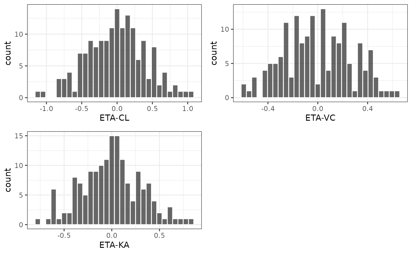

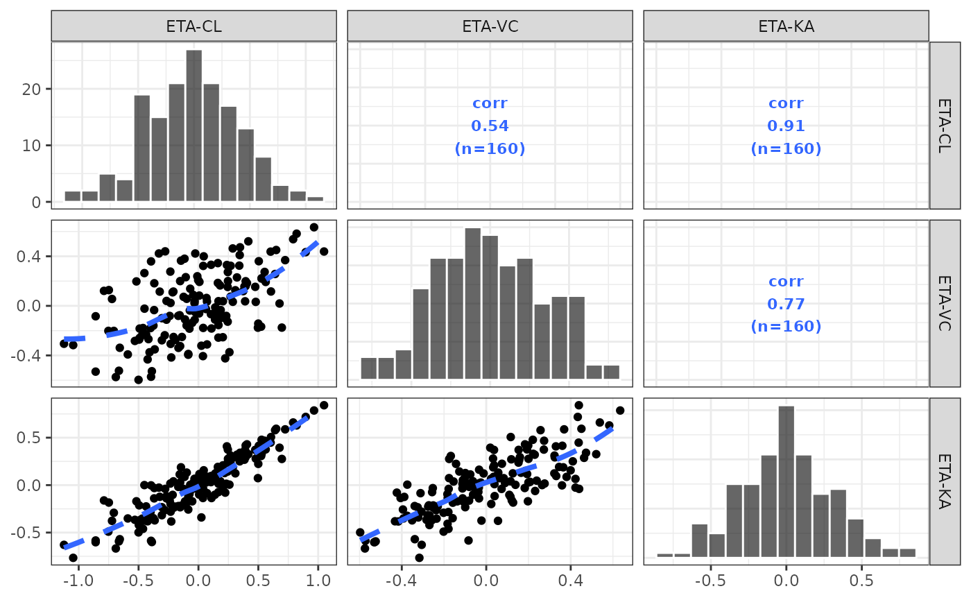
ETA Pairs

eta_pairs(data, etas)

## Loading required namespace: GGally

## Registered S3 method overwritten by 'GGally':
##   method from   
##   +.gg   ggplot2

## `geom_smooth()` using formula 'y ~ x'
## `geom_smooth()` using formula 'y ~ x'
## `geom_smooth()` using formula 'y ~ x'

ETA versus categorical variable

eta_cat(data, x = "STUDYc", y = etas) %>% pm_grid()

ETA versus continuous variable

eta_cont(data, x = "WT", y = etas) %>% pm_grid()

## `geom_smooth()` using formula 'y ~ x'
## `geom_smooth()` using formula 'y ~ x'
## `geom_smooth()` using formula 'y ~ x'