Available functions: pmplots

Kyle Baron

2021-09-13

Setup and packages

library(pmplots)
library(dplyr)
library(purrr)

Example data in the package

df <- pmplots_data_obs() %>% mutate(CWRES = CWRESI)

id <- pmplots_data_id()

dayx <- defx(breaks = seq(0,168,24))

.yname <- "MRG1557 (ng/mL)"

etas <- c("ETA1//ETA-CL", "ETA2//ETA-V2", "ETA3//ETA-KA")

covs <- c("WT//Weight (kg)", "ALB//Albumin (g/dL)", "SCR//Creatinine (mg/dL)")

Override the df and id objects in the above chunk

## Nothing here

col//title specification

This is a way to specify the column name for source data along with the axis label

col_label("CL//Clearance (L)")

. [1] "CL"            "Clearance (L)"

When only the column is given, then the column name will be used for the column title:

col_label("WT")

. [1] "WT" "WT"

Generate using the yspec package

You can also pull col//title data from a yspec object. Load the yspec package and generate an example data specification object

library(yspec)
spec <- ys_help$spec()

Typically, you’ll want to select a subset of columns and then call axis_col_labs()

spec %>% 
  ys_select(WT, AGE, BMI) %>% 
  axis_col_labs()

.                 WT                AGE                BMI 
.  "WT//weight (kg)" "AGE//age (years)" "BMI//BMI (m2/kg)"

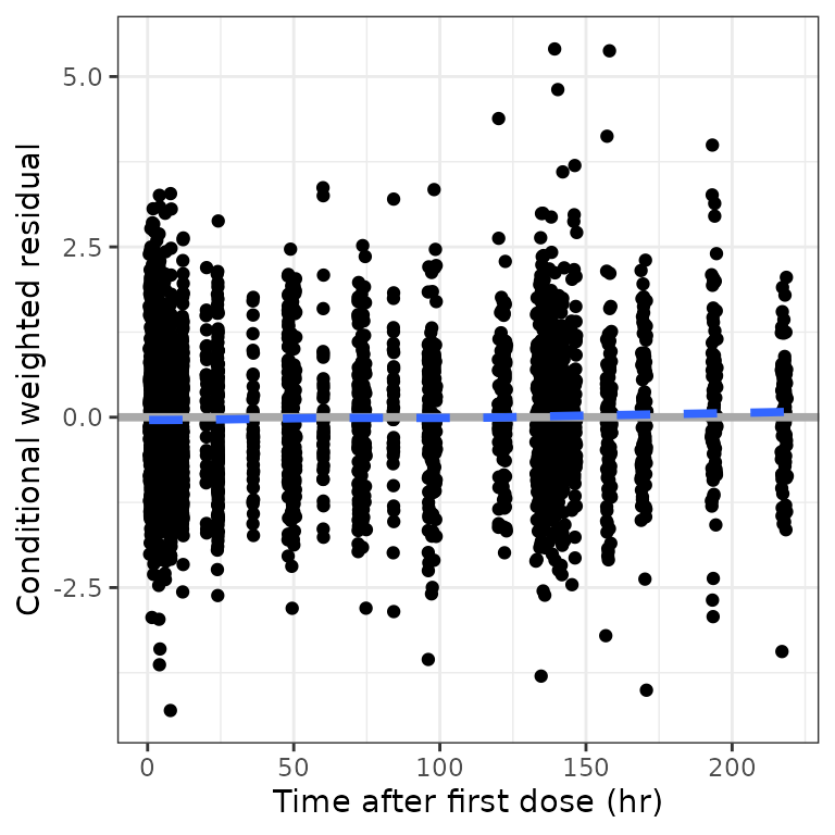
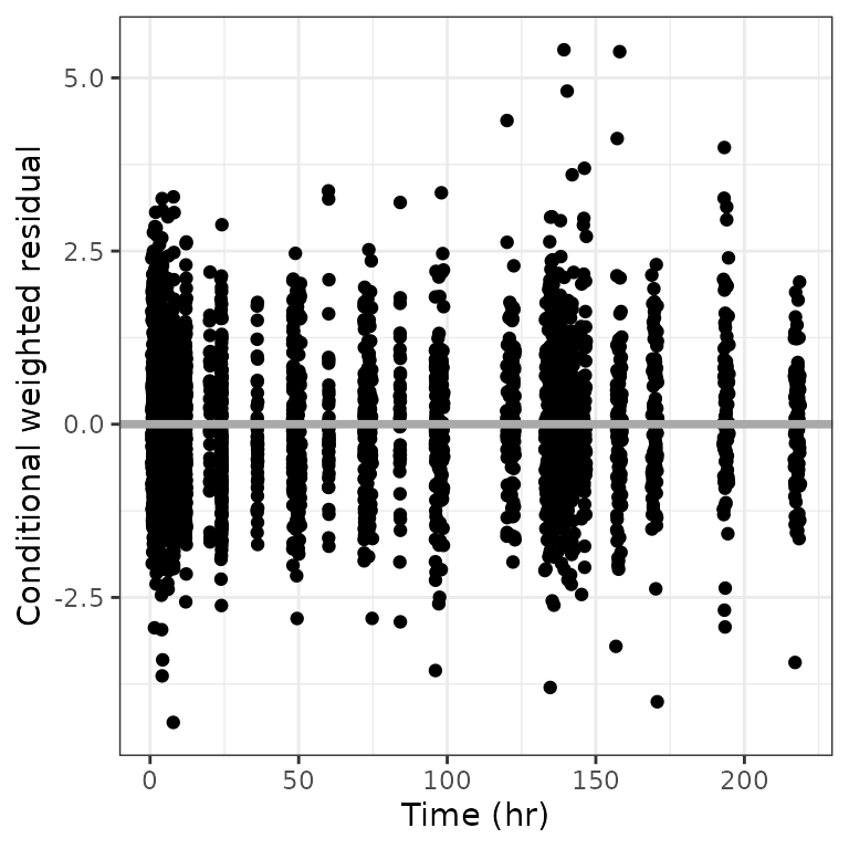
Fill in CWRES if it doesn’t exist

dat <- mutate(df, CWRES = NULL)

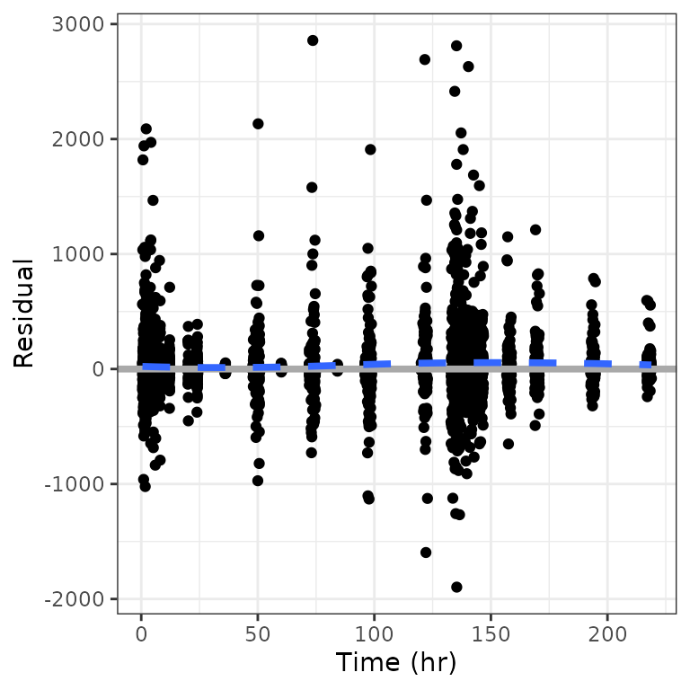
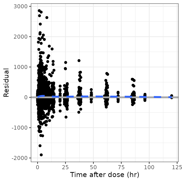
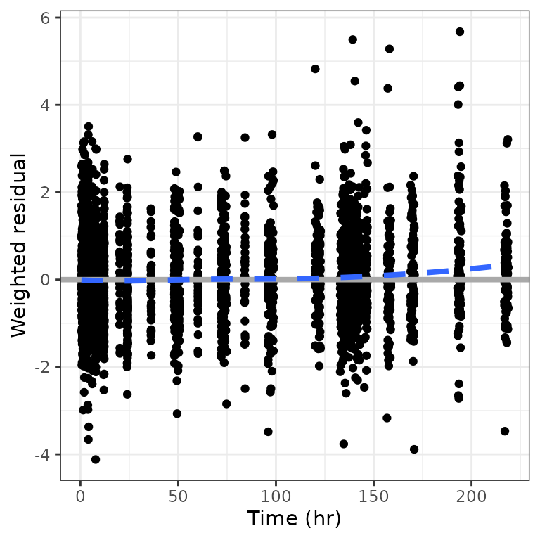
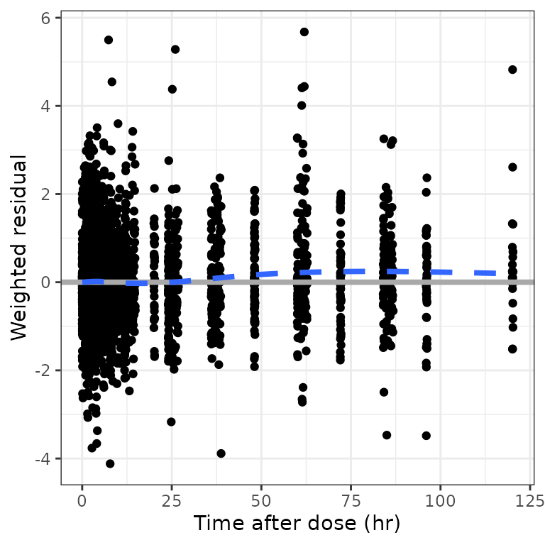
cwresi_time(df)

. `geom_smooth()` using formula 'y ~ x'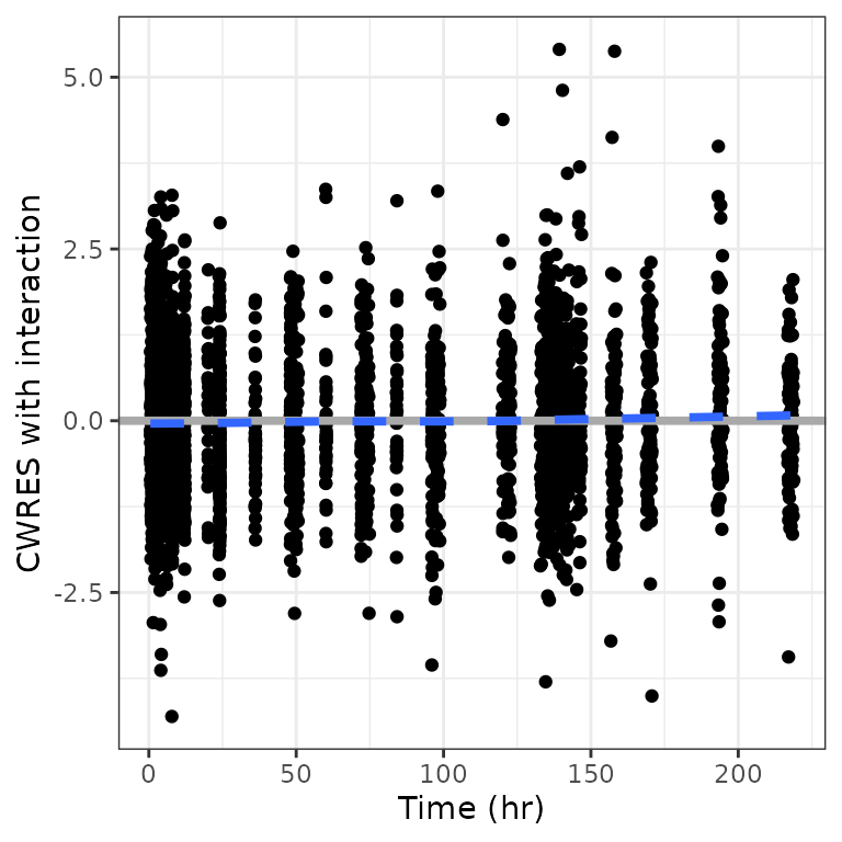

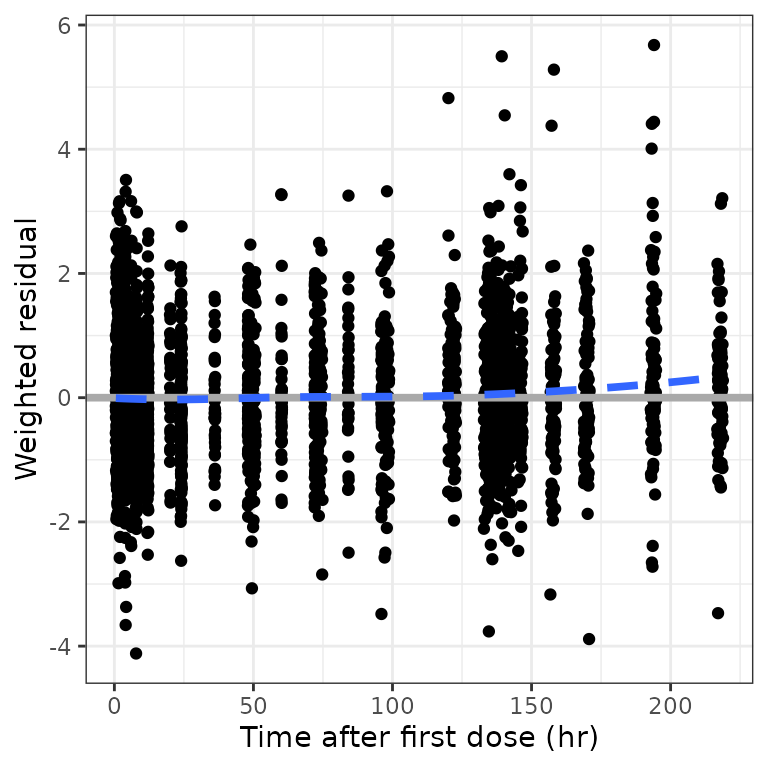
cwres_time(dat)

. Creating CWRES column from CWRESI
. `geom_smooth()` using formula 'y ~ x'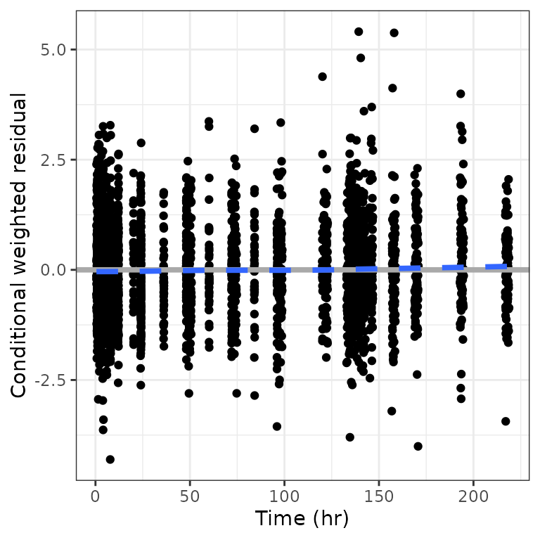

Observed vs predicted

Observed versus population predicted (dv_pred)

dv_pred(df, yname = .yname)

Observed versus population predicted - log/log

dv_pred(df, loglog=TRUE, yname = .yname)

Observed versus individual predicted (dv_ipred)

dv_ipred(df, yname=.yname)

Observed versus individual predicted - log/log

dv_ipred(df, loglog=TRUE, yname = .yname)

Observed versus both PRED and IPRED

dv_preds(df) %>% pm_grid(ncol=2)

Residual plots

Residuals versus time (res_time)

res_time(df)

Residuals versus time after first dose (res_tafd)

res_tafd(df)

Residuals versus time after dose (res_tad)

res_tad(df)

Residuals versus population predicted (res_pred)

res_pred(df)

RES versus continuous covariate (res_cont)

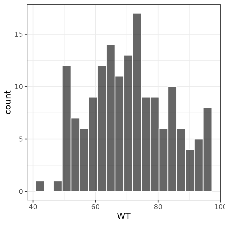
res_cont(df, x="WT//Weight (kg)")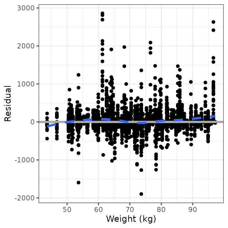

This function is also vectorized in x.

c("WT", "CRCL", "AST") %>% map(.f = partial(res_cont,df)) %>% pm_grid()

RES by categorical covariate (res_cat)

dplyr::count(df, STUDYc)

. # A tibble: 4 × 2
.   STUDYc      n
.   <fct>   <int>
. 1 SAD       424
. 2 MAD      1199
. 3 Renal     960
. 4 Hepatic   559

res_cat(df, x="STUDYc//Study type")

Residual histogram (res_hist)

res_hist(df)

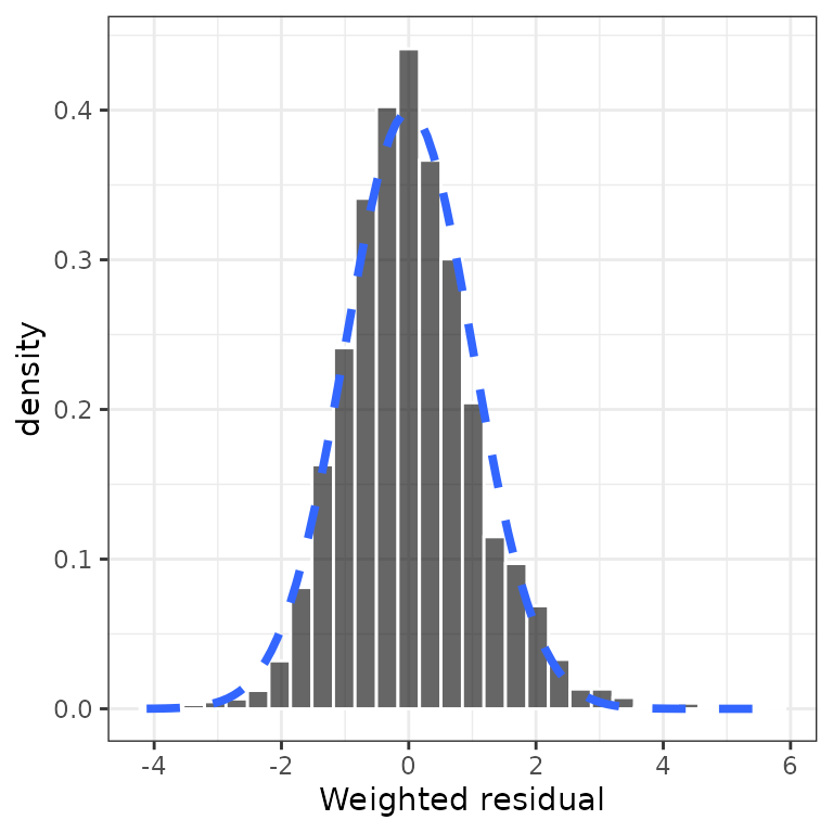
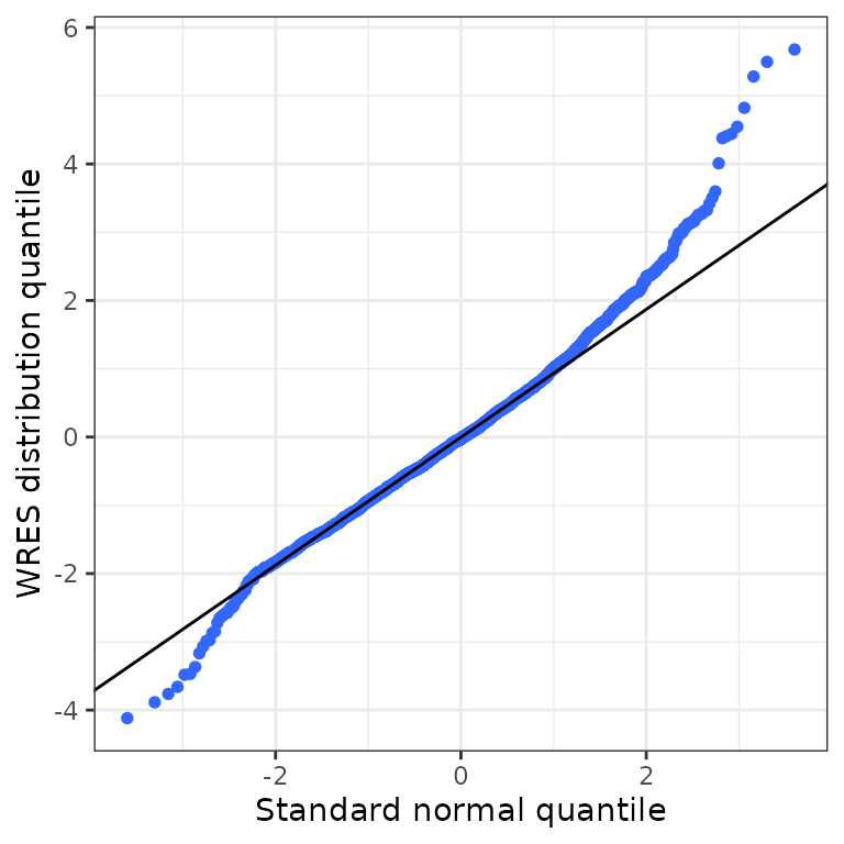
Weighted residuals

Weighted residuals versus time (wres_time)

wres_time(df) 

Weighted residuals versus time after first dose (wres_tafd)

wres_tafd(df)

Weighted residuals versus time after dose (wres_tad)

wres_tad(df)

Weighted residuals versus population predicted (wres_pred)

wres_pred(df)

WRES versus continuous covariate (wres_cont)

This function is also vectorized in x.

wres_cont(df, x="WT//Weight (kg)")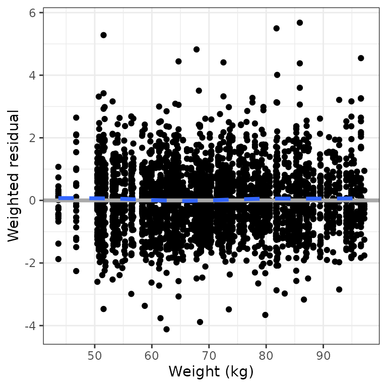

WRES by categorical covariate (wres_cat)

wres_cat(df, x="STUDYc//Study type")

Weighted residual histogram (wres_hist)

wres_hist(df)

WRES QQ plot (wres_q)

wres_q(df)

Conditional weighted residuals (CWRES)

CWRES versus time (cwres_time)

cwres_time(df)

Conditional weighted residuals versus time after first dose (cwres_tafd)

cwres_tafd(df)

CWRES versus time after dose (cwres_tad)

cwres_tad(df)

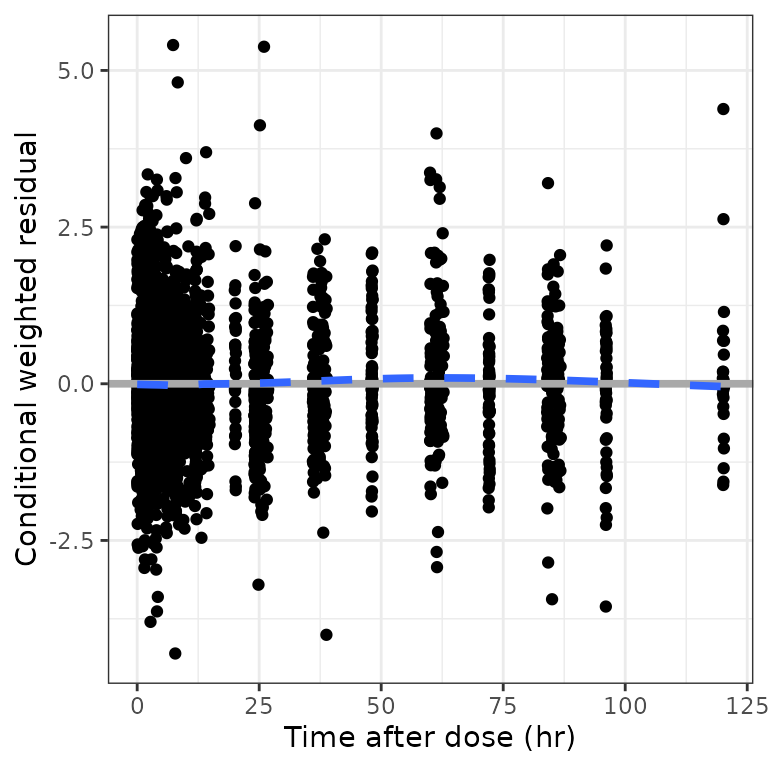
CWRES versus continuous covariate (cwres_cont)

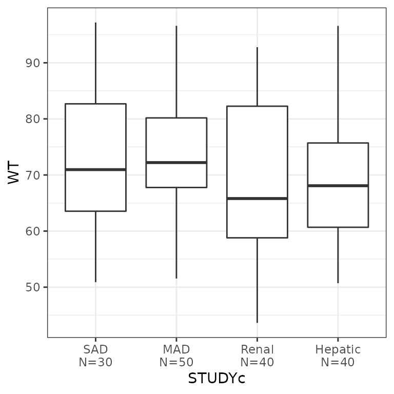
cwres_cont(df, x="WT//Weight (kg)")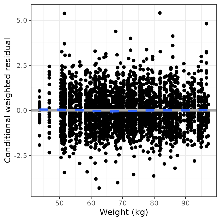

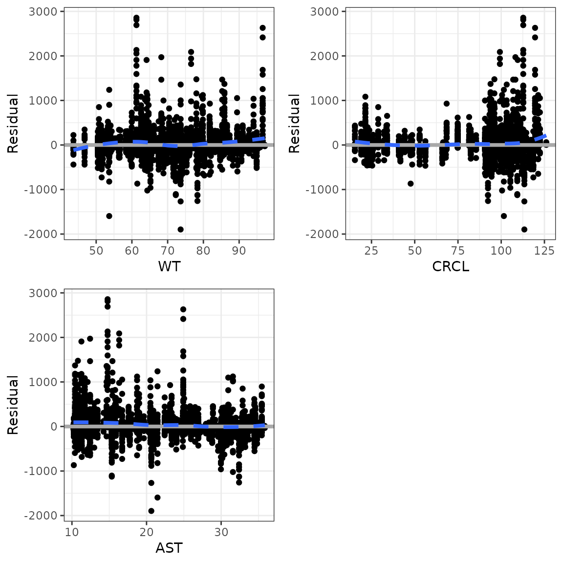
Vectorized version

cwres_cont(df, covs) %>%  pm_grid(ncol=2)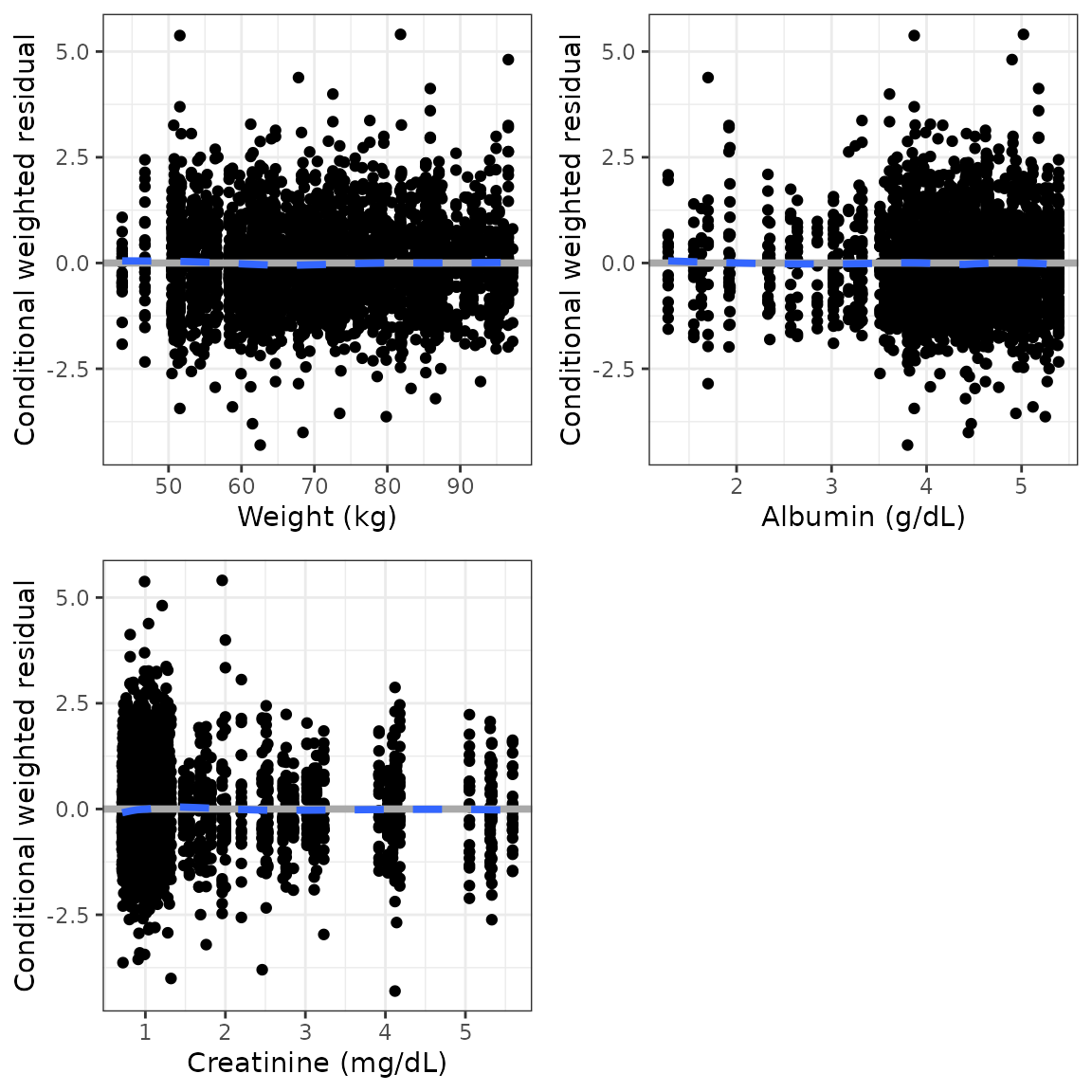

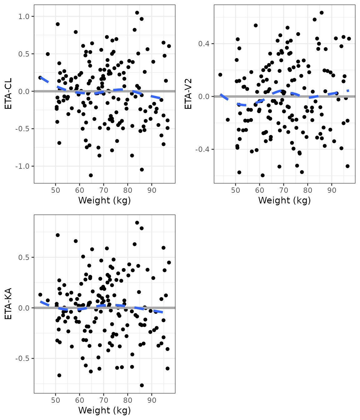
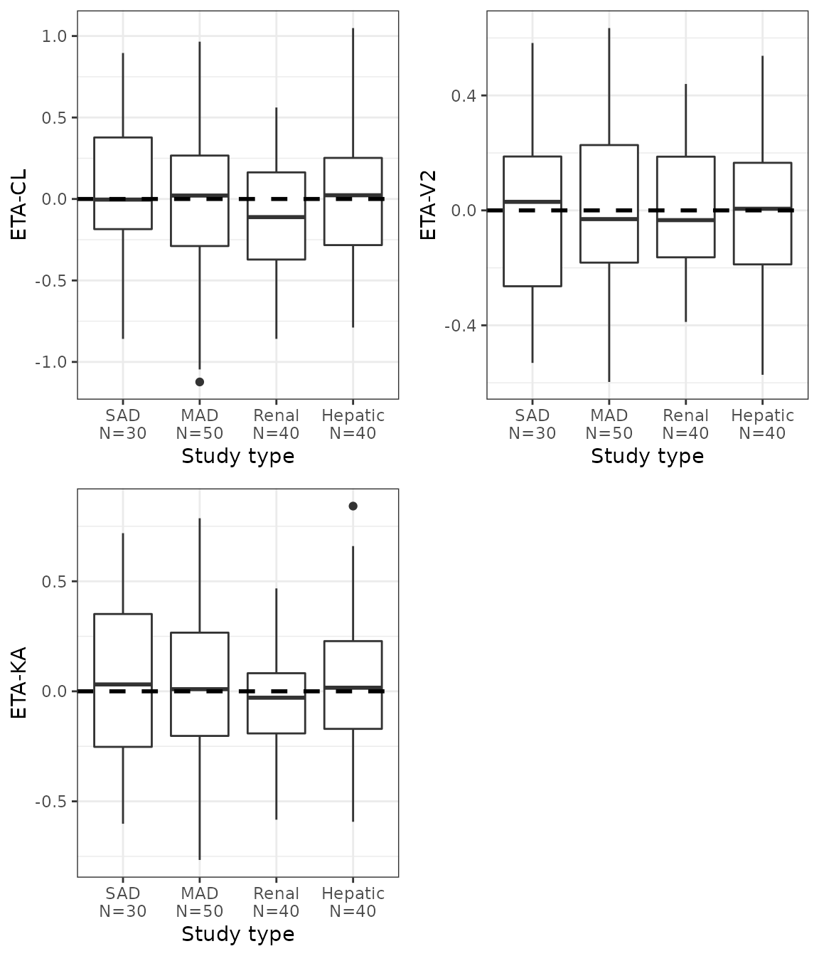
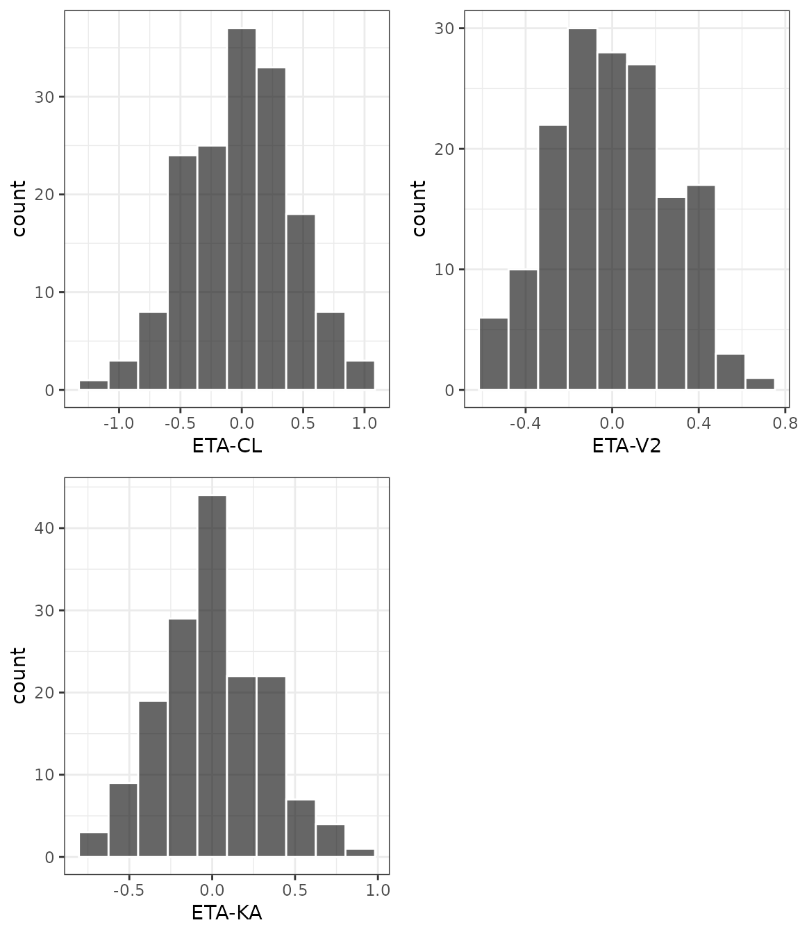
CWRES by categorical covariate (cwres_cat)

cwres_cat(df, x="STUDYc//Study type")

cwres_cat(df, x="STUDYc//Study type", shown=FALSE)

Vectorized version

cwres_cat(df, x = c("STUDYc//Study", "RF//Renal Function"))

. [[1]]

. 
. [[2]]

Conditional weighted residual histogram (cwres_hist)

cwres_hist(df)

CWRES versus population predicted (cwres_pred)

cwres_pred(df)

CWRES QQ plot (cwres_q)

cwres_q(df)

NPDE plots

NPDE versus TIME (npde_time)

npde_time(df)

NPDE versus TAD (npde_tad)

npde_tad(df)

NPDE versus TAFD (npde_tafd)

npde_tafd(df)

NPDE versus PRED (npde_pred)

npde_pred(df)

NPDE versus continuous variable (npde_cont)

npde_cont(df, "WT")

NPDE versus categorical variable (npde_cat)

npde_cat(df, "STUDYc")

QQ-plot with NPDE (npde_q)

npde_q(df)

NPDE histogram (npde_hist)

npde_hist(df)

ETA plots

etas <- c("ETA1//ETA-CL", "ETA2//ETA-V2", "ETA3//ETA-KA")
covs <- c("WT//Weight (kg)", "ALB//Albumin (g/dL)", "SCR//Creatinine (mg/dL)")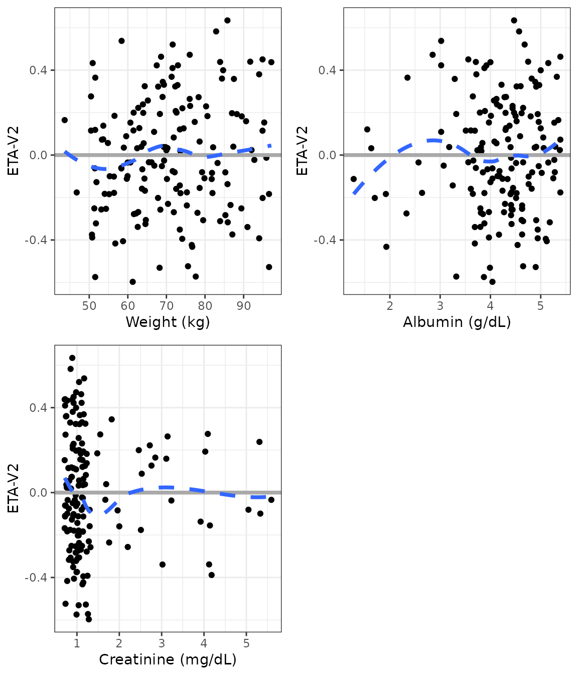

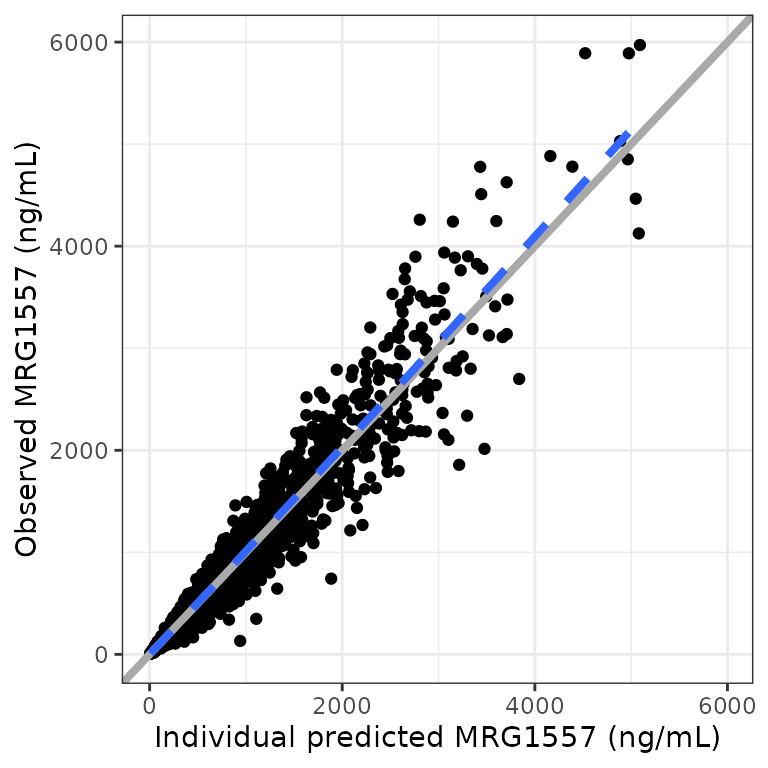
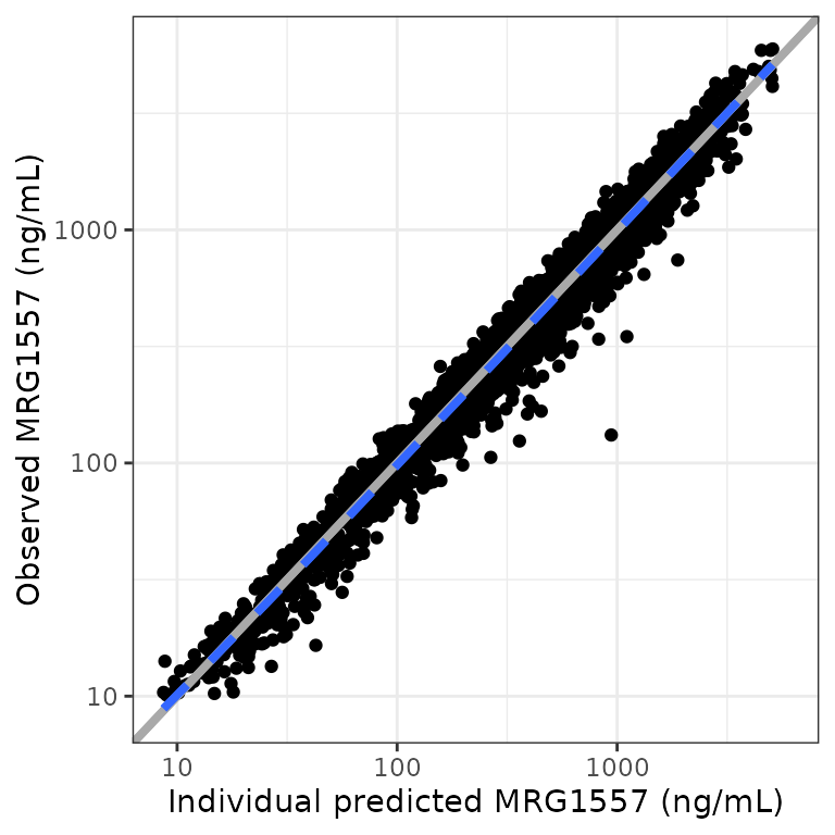
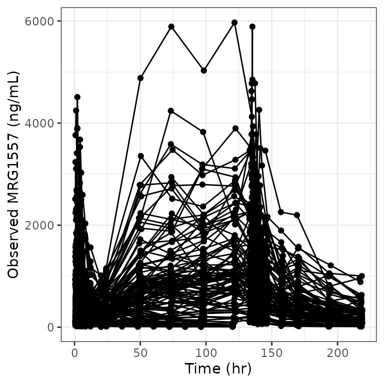
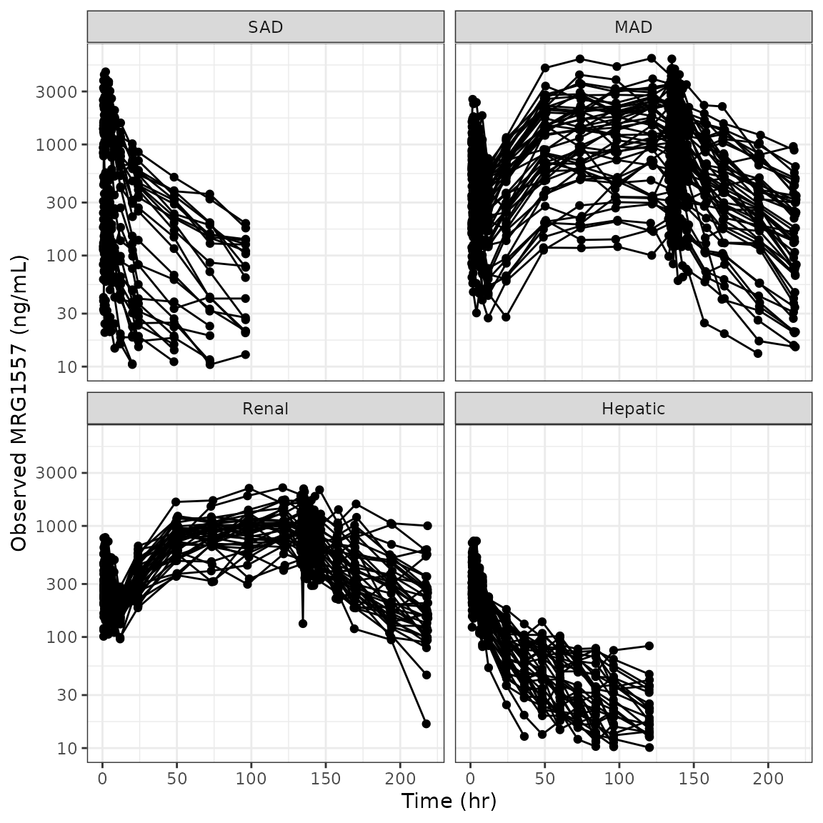
ETA versus continuous covariates (eta_cont)

Grouped by eta

eta_cont(id, x=covs,y=etas[2]) %>% pm_grid()

Grouped by covariate

eta_cont(id, x=covs[1], y=etas) %>% pm_grid(ncol=2)

ETA by categorical covariates (eta_cat)

p <- eta_cat(id, x="STUDYc//Study type", y=etas)

pm_grid(p)

ETA histograms (eta_hist)

etas <- c("ETA1//ETA-CL", "ETA2//ETA-V2", "ETA3//ETA-KA")
p <- eta_hist(id,etas, bins=10)

pm_grid(p)

ETA pairs plot (eta_pairs)

p <- eta_pairs(id, etas)

print(p)

DV versus time (dv_time)

Basic plot

dv_time(df, yname = .yname)

Faceted

dv_time(df, yname="MRG1557 (ng/mL)") + facet_wrap(~DOSE, scales="free_x")

NOTE this will not work as you expect; the labels are wrong.

cwres_cat(df, x = "STUDYc") + facet_wrap(~CPc)

The only way to get this right is

cwres_cat(df, x = "STUDYc", shown=FALSE) + facet_wrap(~CPc)

log-Scale

dv_time(df, yname="MRG1557 (ng/mL)", log=TRUE) + facet_wrap(~STUDYc)

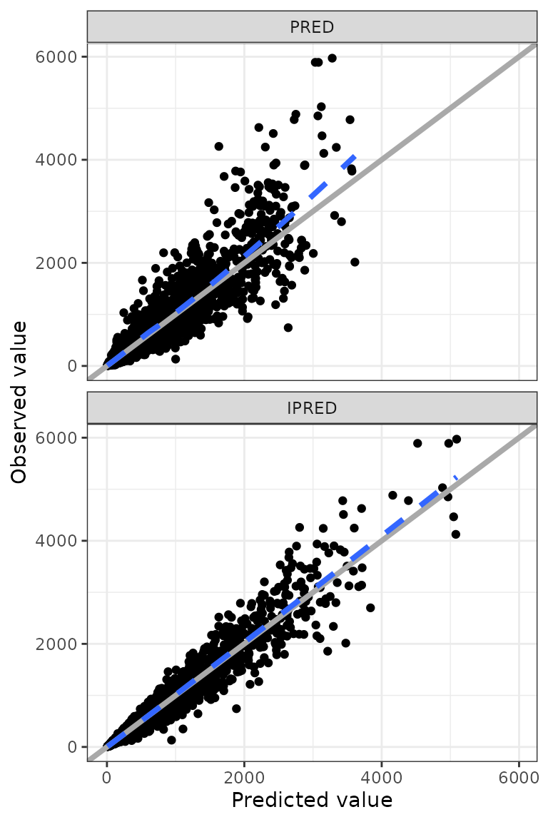
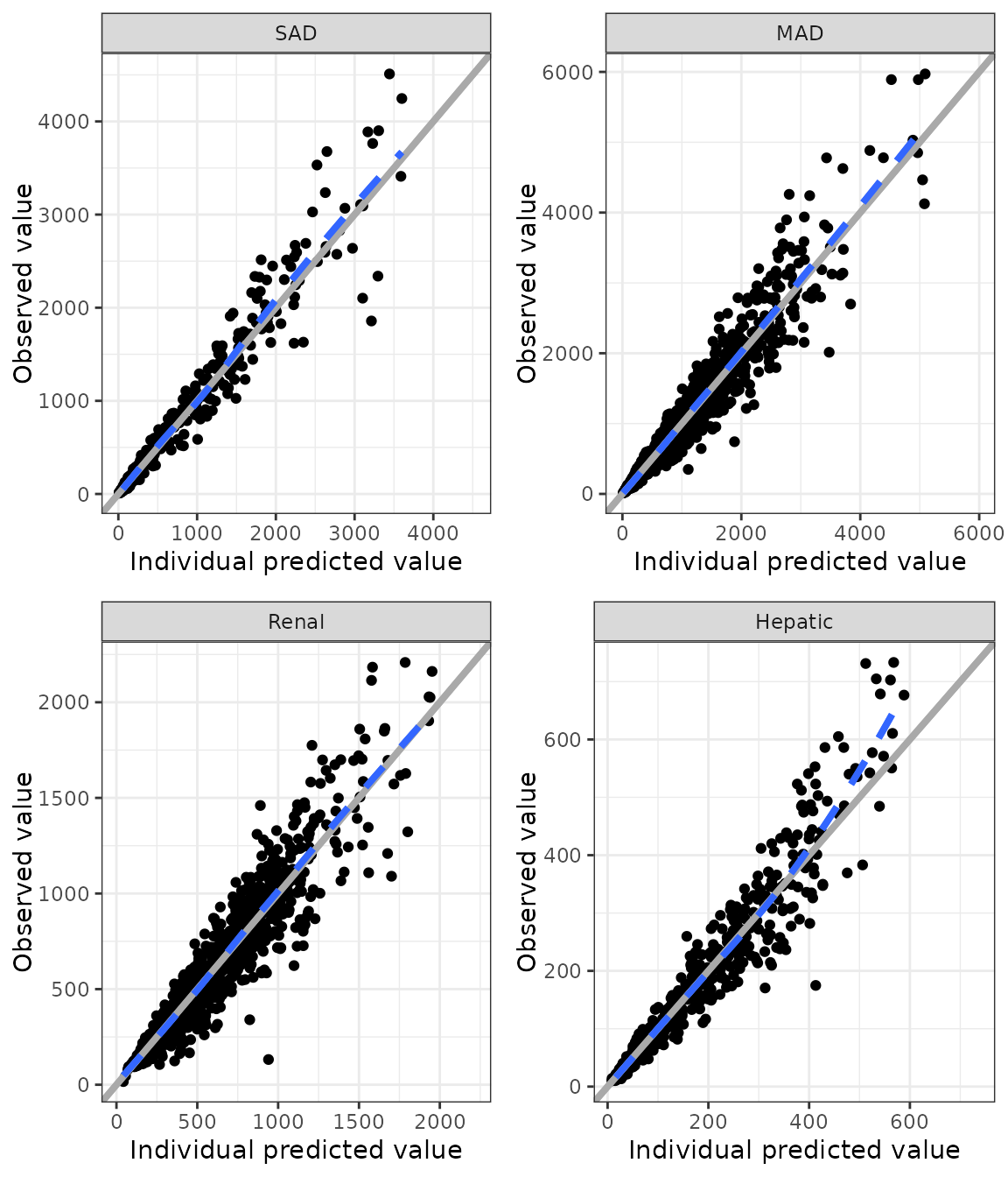
DV-PRED-IPRED

• This returns a list of plots; we show only one here (the first 9 IDs) as an example

dd1 <- filter(df, ID <= 15)

dv_pred_ipred(dd1, nrow = 3, ncol = 3, ylab = "Concentration (ng/mL)", log_y=TRUE)

. $`1`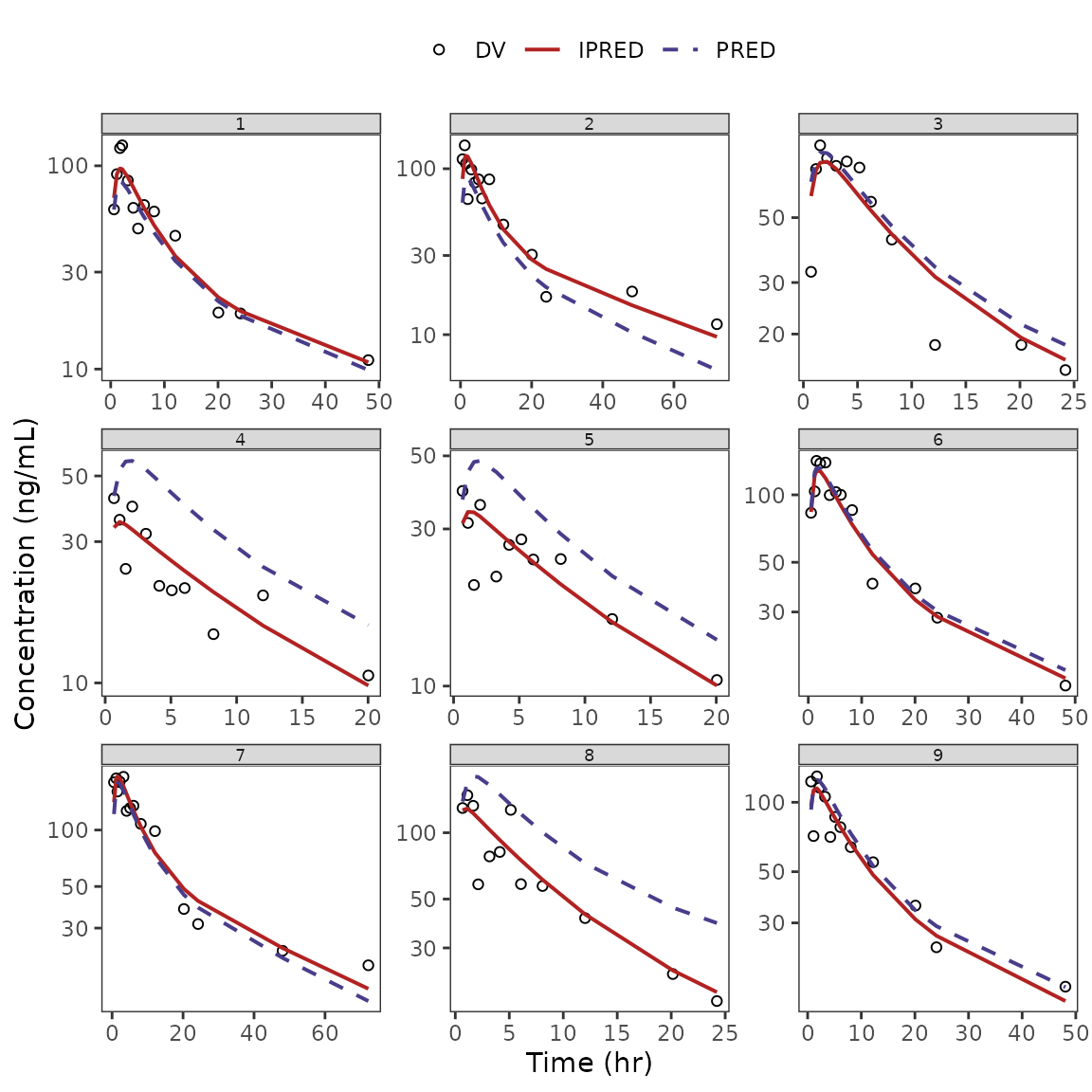

. 
. $`2`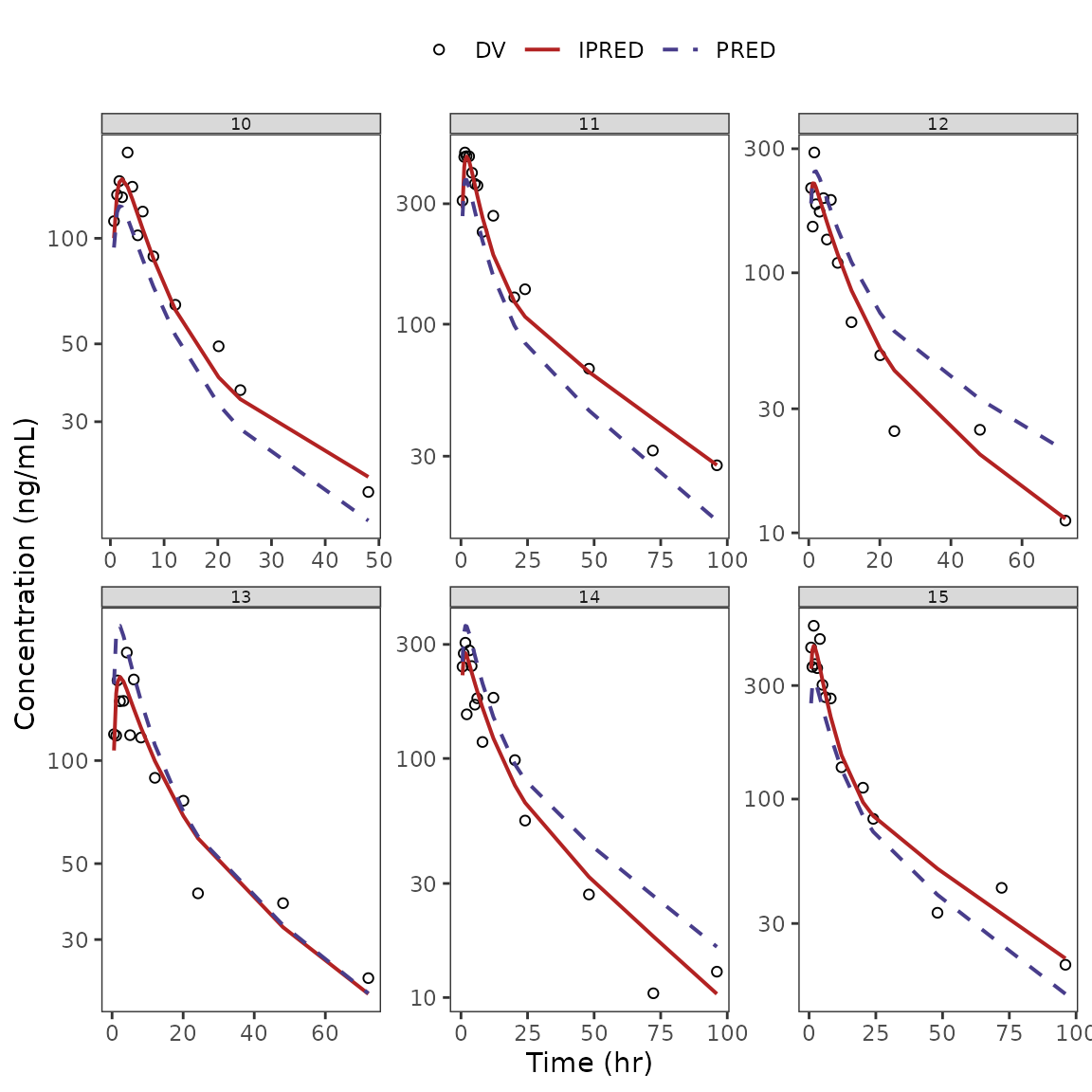

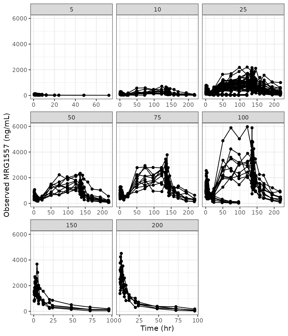
Wrapped plots

Histogram

wrap_hist(df, x = c("WT", "ALB", "SCR"), scales = "free", bins=10, ncol=2)

ETA versus continuous

wrap_eta_cont(df, y = "ETA1", x = c("WT", "ALB"), scales="free_x")

Continuous on categorical

wrap_cont_cat(df, y = c("WT", "CRCL", "AAG"), x = "STUDYc", ncol = 2) 

Continuous on continuous

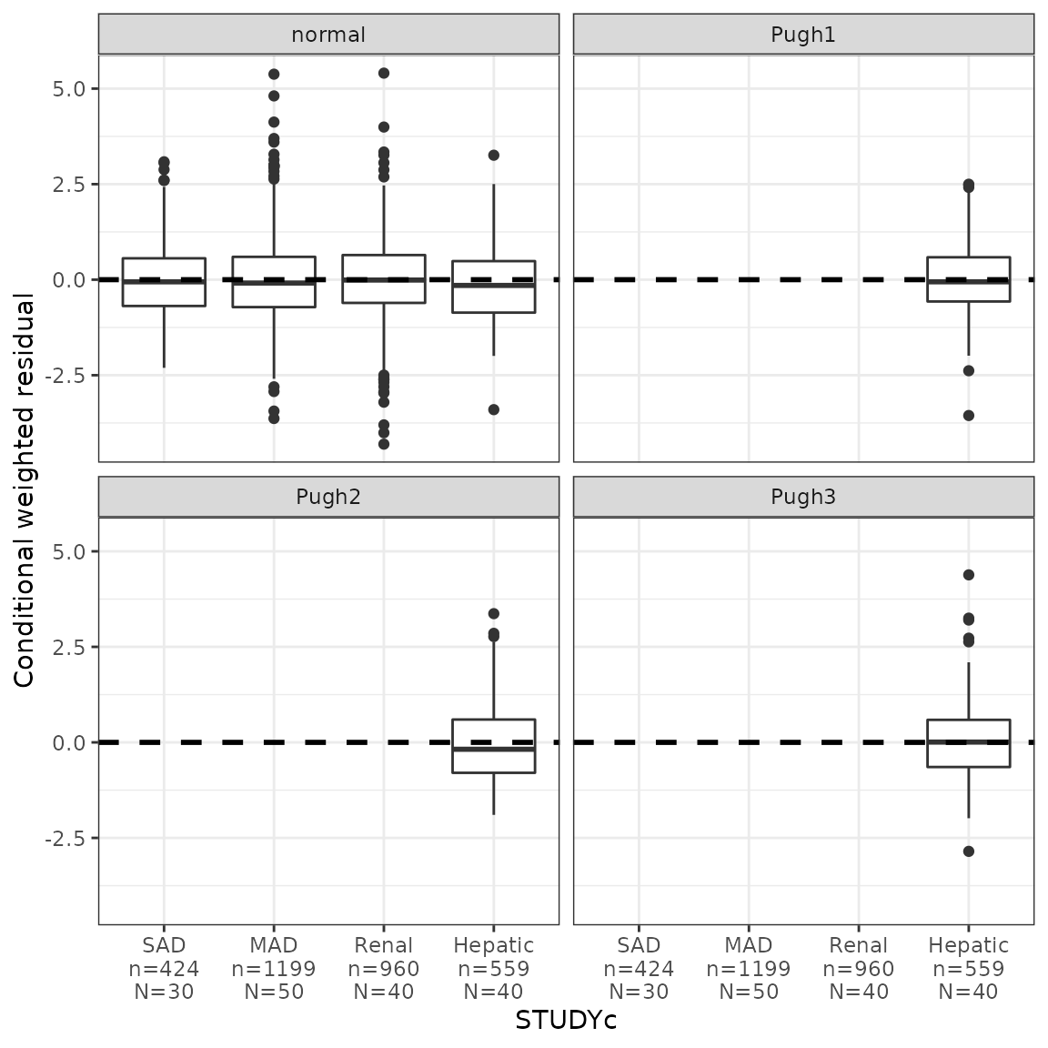
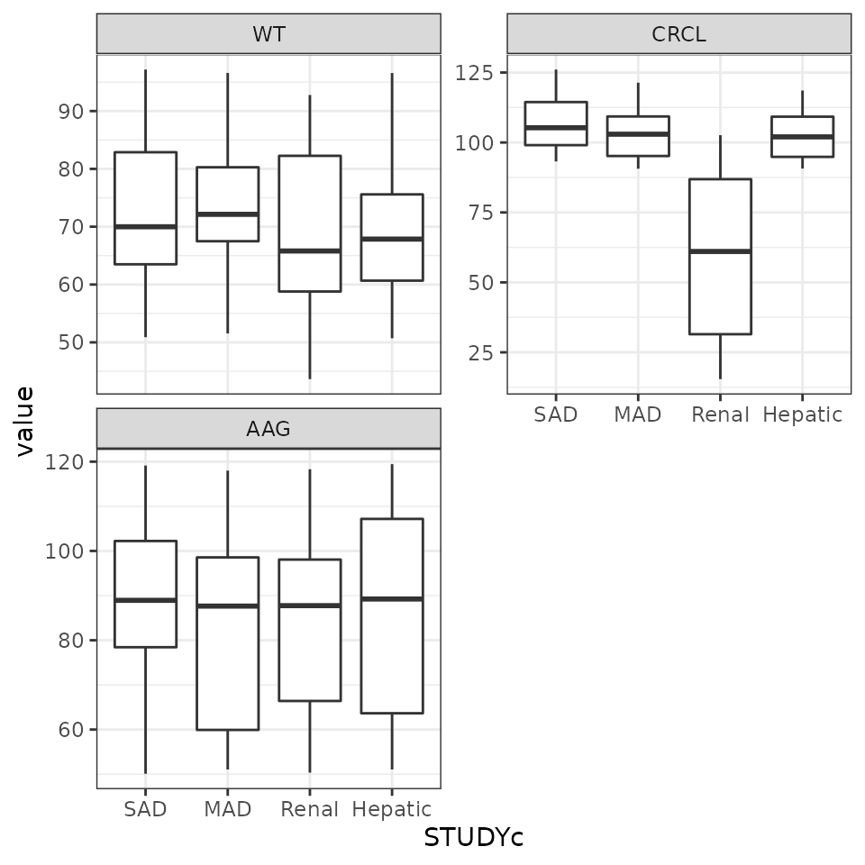
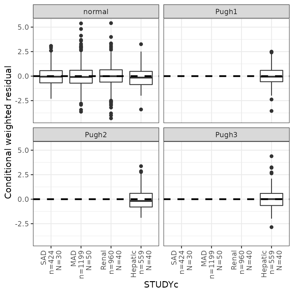
wrap_cont_cont(df, y = "CWRES" , x = c("WT", "CRCL", "AAG"), ncol = 2, scales="free_x")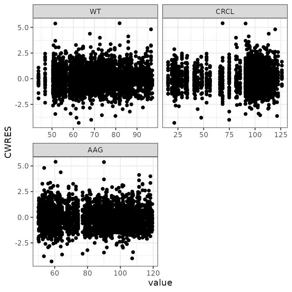 

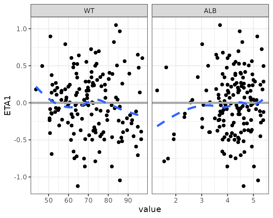
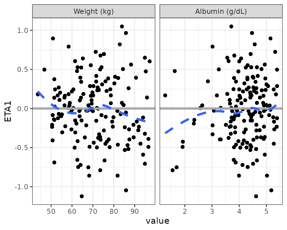
Residuals versus time

wrap_res_time(df, y = c("RES", "WRES", "CWRES"), ncol = 2, scales="free_y") 

DV/PRED and DV/IPRED

wrap_dv_preds(df, ncol=1)

Use labels in the strip

wrap_eta_cont(
  df, 
  y = "ETA1", 
  x = c("WT//Weight (kg)", "ALB//Albumin (g/dL)"),
  scales="free_x", 
  use_labels=TRUE
)

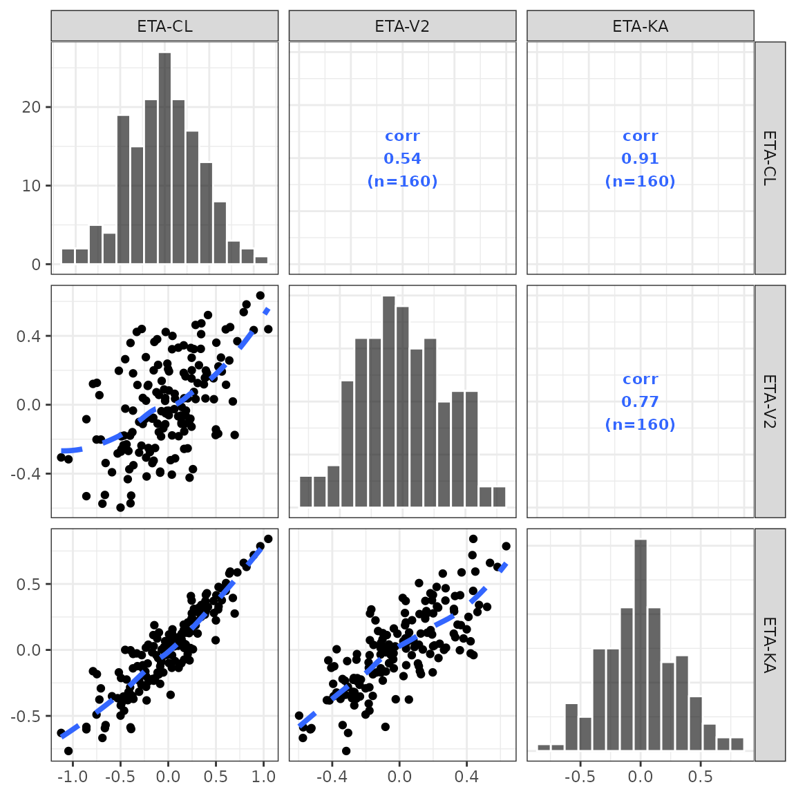
Pairs plots

This is a simple wrapper around GGally::ggpairs with some customizations that have been developed internally at Metrum over the years.

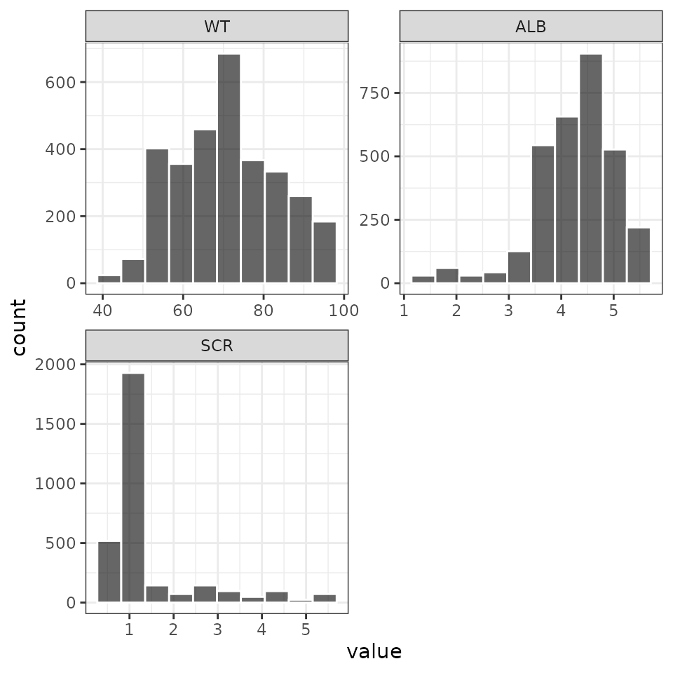
pairs_plot(id, c("WT//Weight", "ALB//Albumin", "SCR//Serum creat"))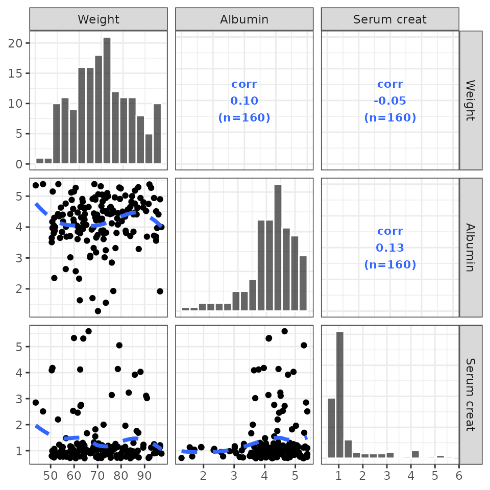

Customized lower triangle

Pass a function that customizes the scatter plots on the lower triangle. This function should accept a gg object and add a geom to it

my_lower <- function(p) {
  p + geom_point(aes(color = STUDYc)) + 
    geom_smooth(se = FALSE, color = "black")
}

pairs_plot(id, c("WT", "ALB"), lower_plot = my_lower)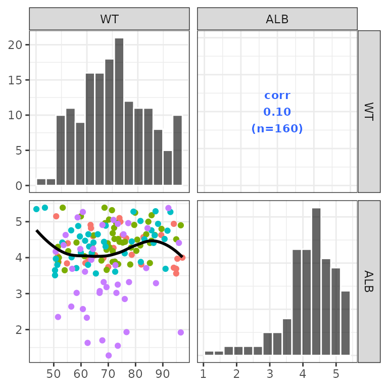

Vectorized plots

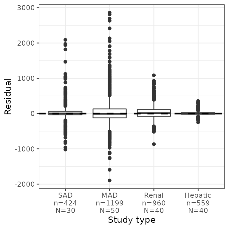
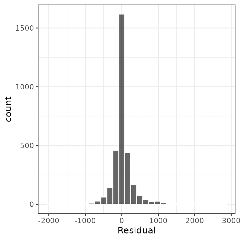
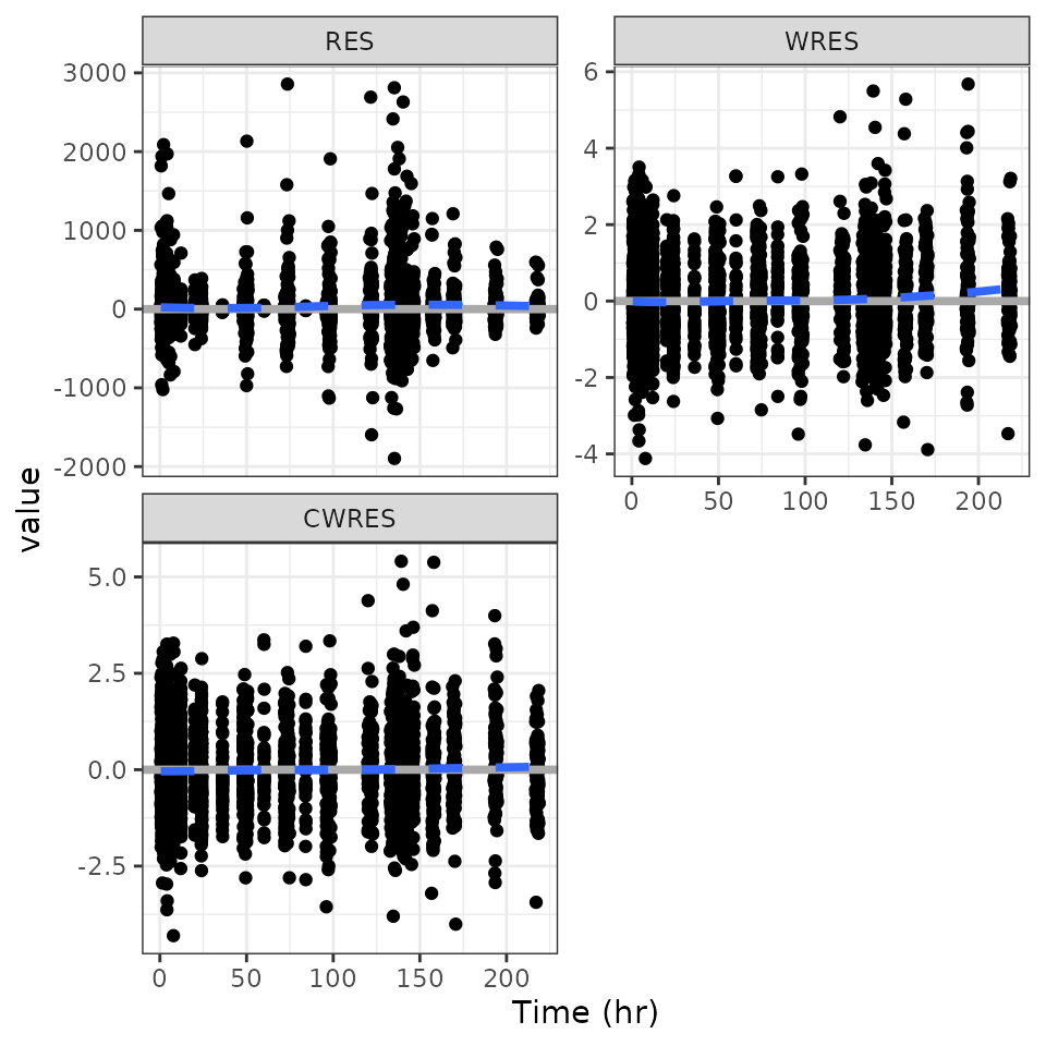
pm_scatter(df, x = "TIME", y = c("RES", "WRES", "CWRES"))

. [[1]]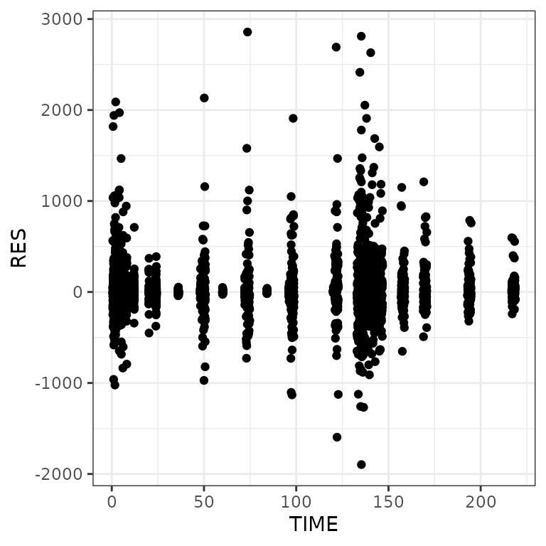

. 
. [[2]]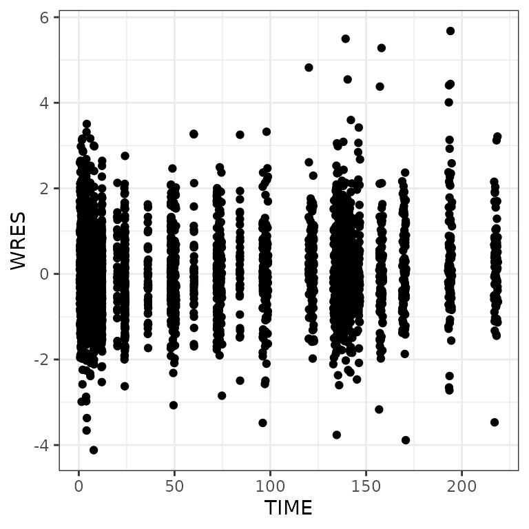

. 
. [[3]]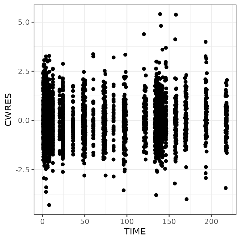

Data summary

Continuous variable by categorical variable (cont_cat)

cont_cat(id, x="STUDYc", y="WT")

General histogram (cont_hist)

cont_hist(id, x = "WT", bins = 20)

Split and plot (split_plot)

p <- split_plot(df, sp="STUDYc", fun=dv_ipred)

pm_grid(p)

Some customization

Latex (including Greek letters) in axis title

dv_pred(df, x = "PRED//Concentration ($\\mu$g)")

Latex in pairs plot

data <- dplyr::tibble(m = rnorm(100), s = rnorm(100), n = rnorm(100))

x <- c("m//$\\mu$", "s//$\\sigma$", "n//$\\nu$")

pairs_plot(data,x)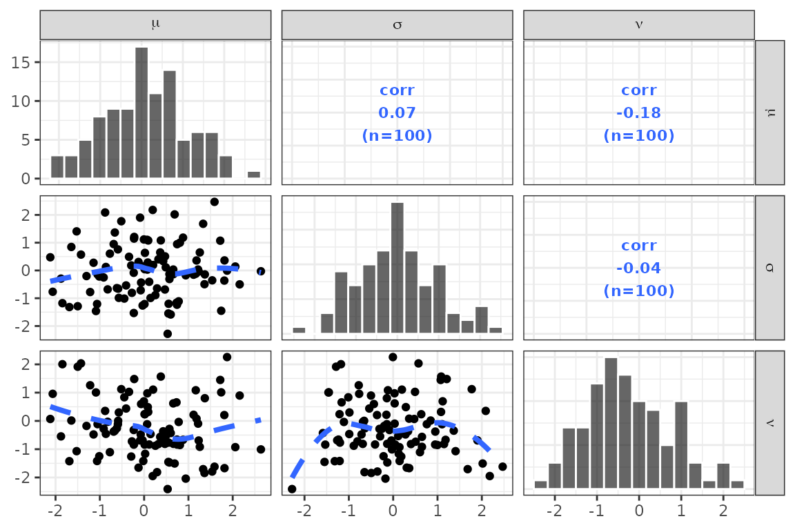

Latex in wrapped plots

y <- c("WT//Weight (kg)", "BMI//BMI (kg/m$^2$)", "SCR//SCR (g/dL)")

wrap_cont_time(df, y = y, use_labels=TRUE)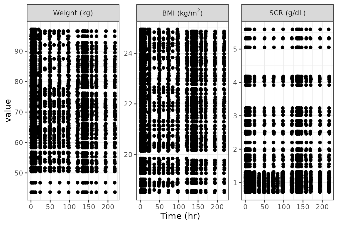

Modify x-axis

a <- list(trans="log", breaks = logbr3())

dv_time(df, xs=a)

Modify y-axis

dv_time(df, ys=a, yname="Y-axis name")

Flip coordinates when labels get cramped

If this is too cramped

cont_cat(
  id, 
  y = c("WT", "BMI", "ALB", "CRCL"), 
  x = "STUDYc"
) %>% pm_grid()

Try this

cont_cat(
  id, 
  y = c("WT", "BMI", "ALB", "CRCL"), 
  x = "STUDYc"
) %>% map(~.x+coord_flip()) %>% pm_grid()

Add layers

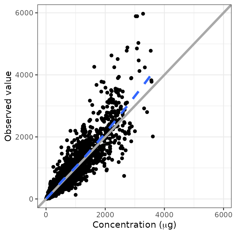
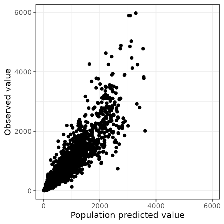
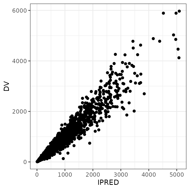
p <- ggplot(df, aes(PRED,DV))  + geom_point() + pm_theme()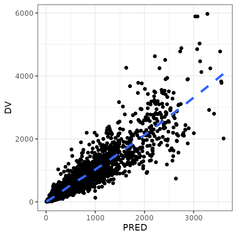

smooth

layer_s(p)

abline

layer_a(p)

layer_h(cwres_time(df,add_layers=FALSE))

Drop extra layers

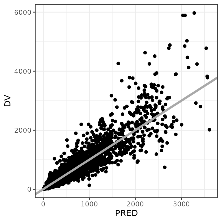
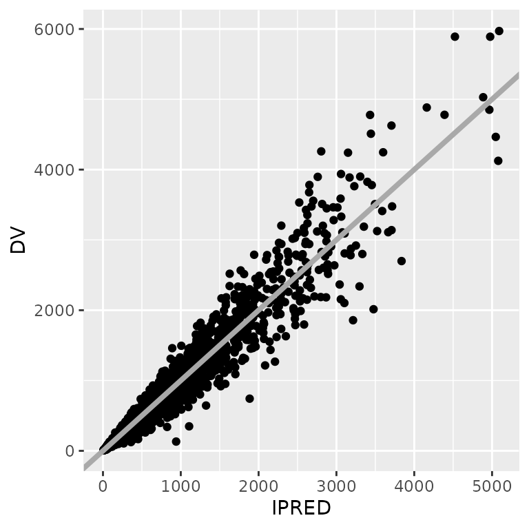
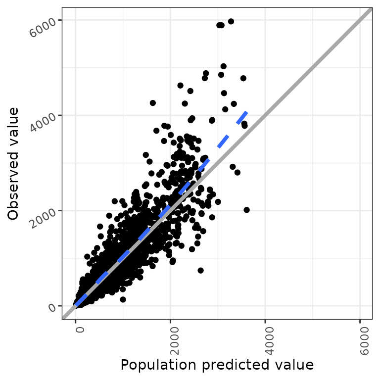
dv_pred(df, smooth=NULL)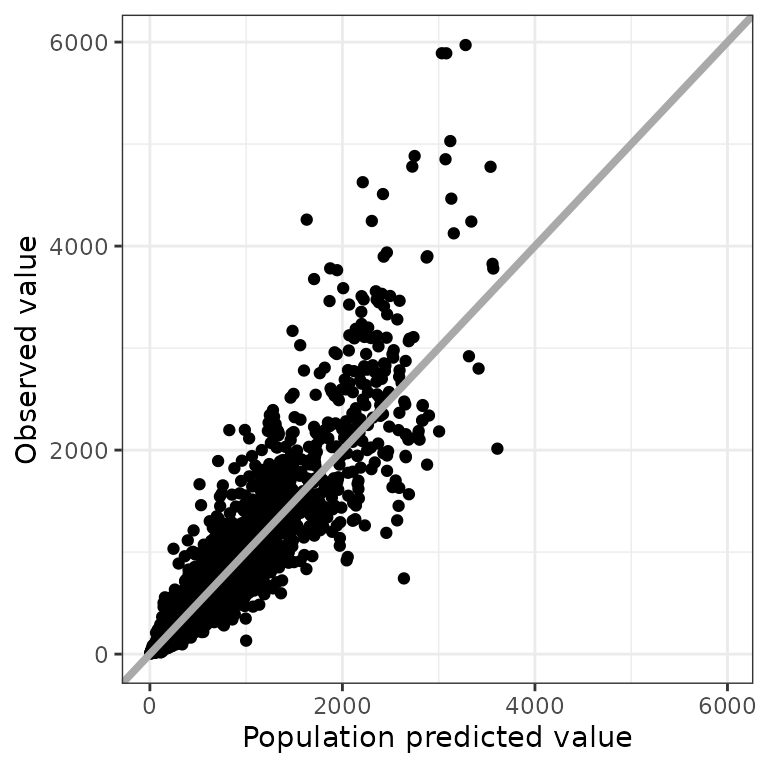

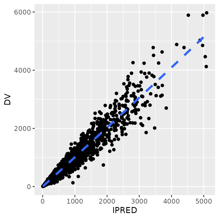
dv_pred(df, abline=NULL)

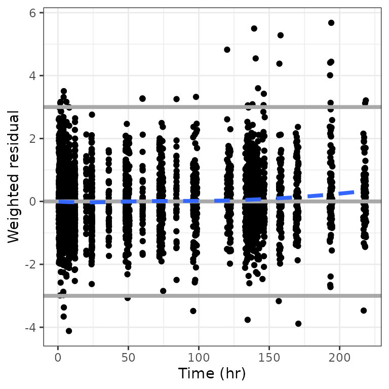
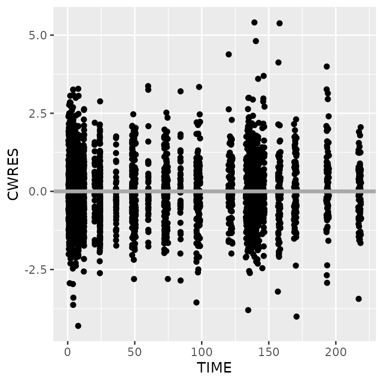
cwres_time(df, hline = NULL)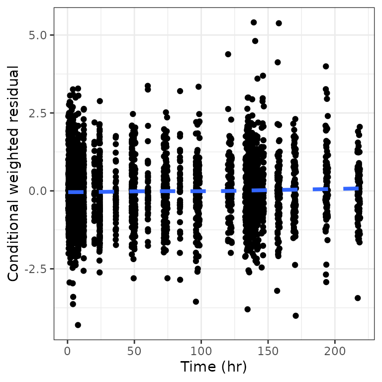

dv_pred(df, abline=NULL, smooth = NULL)

Modify layer specs

For example, change the values of argument for geom_smooth

cwres_time(df, smooth = list(method = "loess", span = 0.1, se=TRUE))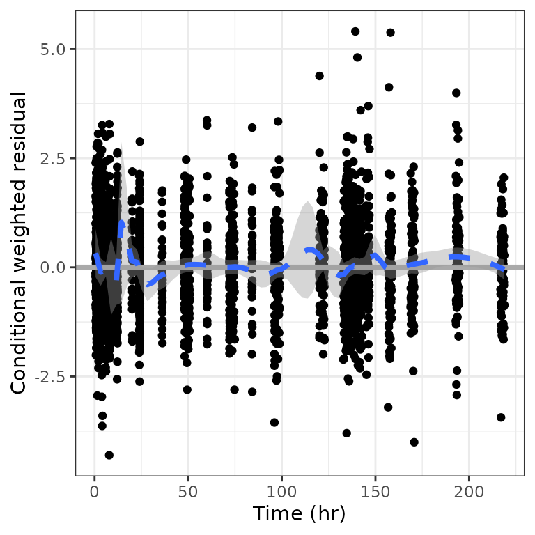

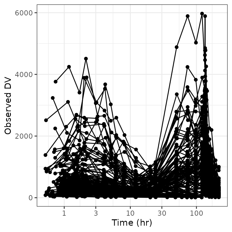
Drop all extra layers

dv_pred(df, add_layers=FALSE)

Custom breaks

Default breaks:

dv_time(df)

Break every 3 days

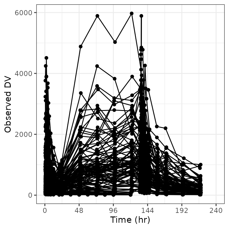
dv_time(df, xby=72)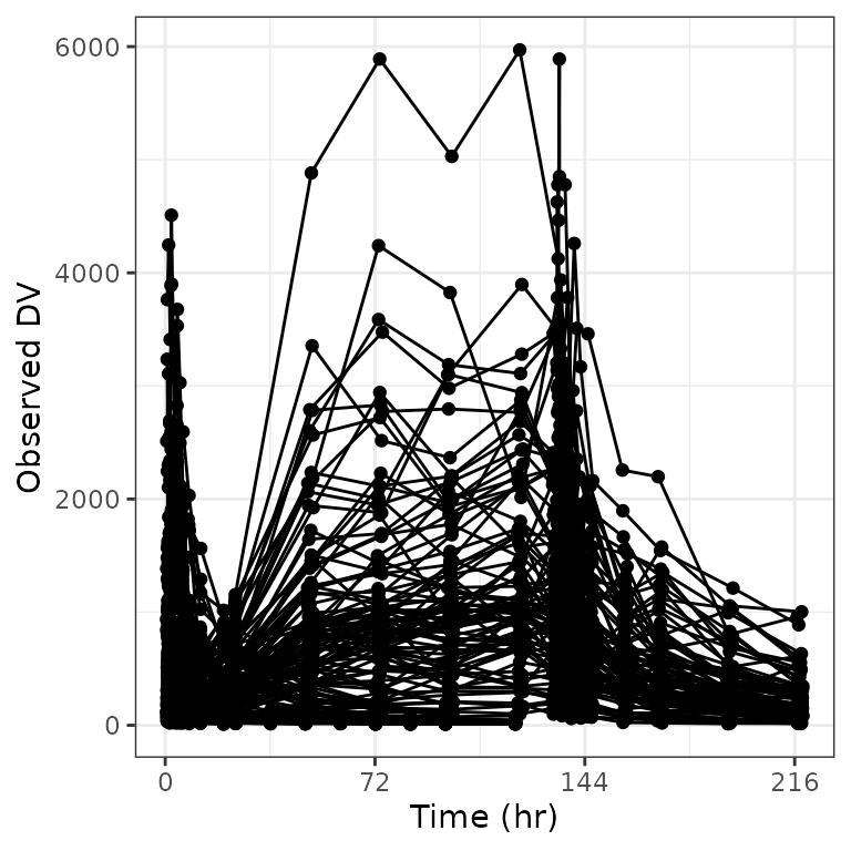

Custom breaks and limits

a <- list(breaks = seq(0,240,48), limits=c(0,240))
dv_time(df, xs=a)

Extra reference lines to [C]WRES plots

wres_time(df) + geom_3s()

Replicate look and feel

p <- ggplot(df, aes(IPRED,DV)) + geom_point()

p

Theme

p + pm_theme()

Plain

p + theme_plain()

Smooth

p + pm_smooth()

Abline

p + pm_abline()

Horizontal reference line

ggplot(df, aes(TIME,CWRES)) + geom_point() + pm_hline()

Rotate x and y axis labels

Specify the angle

dv_pred(df) + rot_x(angle = 90) + rot_y()

Rotate to vertical

We are typically rotating the tick labels on the x-axis and frequently it is convenient to ask for a totally vertical rendering

cwres_cat(df, x = "STUDYc") + 
  facet_wrap(~CPc) + rot_x(vertical = TRUE)

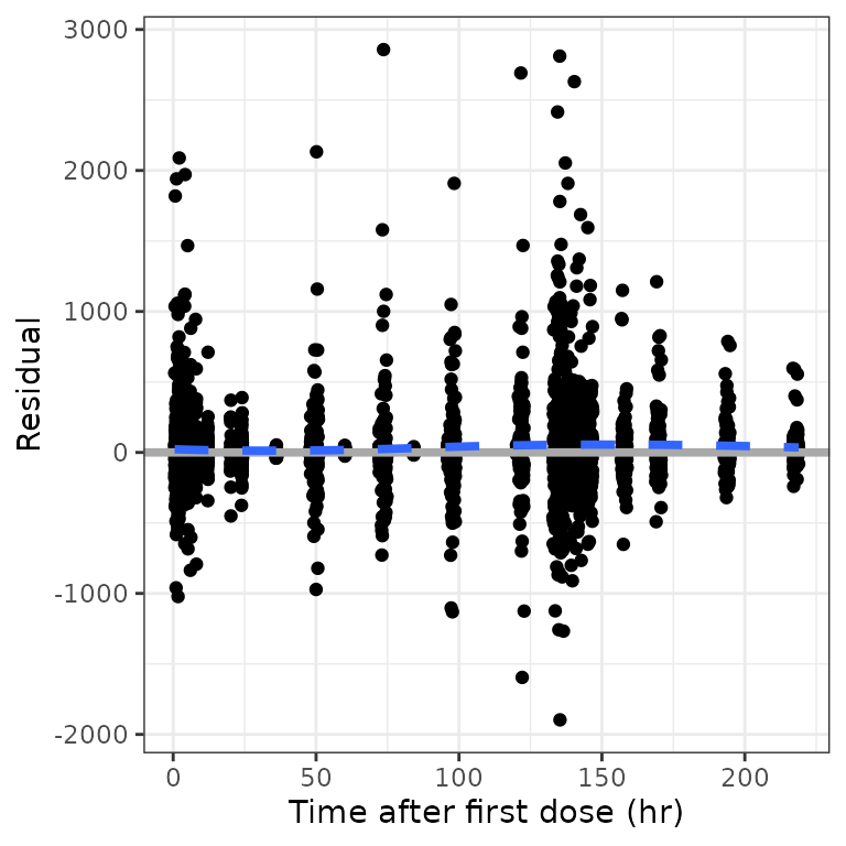
Standard axis titles

pm_axis_time()

. [1] "TIME//Time {xunit}"

pm_axis_tad()

. [1] "TAD//Time after dose {xunit}"

pm_axis_tafd()

. [1] "TAFD//Time after first dose {xunit}"

pm_axis_res()

. [1] "RES//Residual"

pm_axis_wres()

. [1] "WRES//Weighted residual"

pm_axis_cwres()

. [1] "CWRES//Conditional weighted residual"

pm_axis_cwresi()

. [1] "CWRESI//CWRES with interaction"

pm_axis_npde()

. [1] "NPDE//NPDE"

pm_axis_dv()

. [1] "DV//Observed {yname}"

pm_axis_pred()

. [1] "PRED//Population predicted {xname}"

pm_axis_ipred()

. [1] "IPRED//Individual predicted {xname}"

Log breaks

logbr3()

.  [1] 1e-10 3e-10 1e-09 3e-09 1e-08 3e-08 1e-07 3e-07 1e-06 3e-06 1e-05 3e-05
. [13] 1e-04 3e-04 1e-03 3e-03 1e-02 3e-02 1e-01 3e-01 1e+00 3e+00 1e+01 3e+01
. [25] 1e+02 3e+02 1e+03 3e+03 1e+04 3e+04 1e+05 3e+05 1e+06 3e+06 1e+07 3e+07
. [37] 1e+08 3e+08 1e+09 3e+09 1e+10 3e+10

logbr()

.  [1] 1e-10 1e-09 1e-08 1e-07 1e-06 1e-05 1e-04 1e-03 1e-02 1e-01 1e+00 1e+01
. [13] 1e+02 1e+03 1e+04 1e+05 1e+06 1e+07 1e+08 1e+09 1e+10